Hello students! We are back. In this week’s reading, you’ll learn how to work with data in R - first how psychologists define data, then how to graph (and think critically about) different types of data with your HUMAN BRAIN, and finally how to work with data (and datasets) in R.
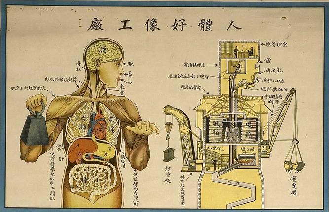
Chinese medical poster, 1933 (ref US NLM; image source here)
ImportantTo-Do List:
Read this document and watch the videos to learn how to…
define different types of data, and using your human brain to understand these data (Part 1 : Statistics)
use R to define variables, import datasets, and navigate these datasets (Part 2 : R)
navigate the big business of academic research, and find research articles relevant to your interests (Part 3 : Research Methods)
Take the practice exam (on navigating and loading datasets) in Part 2.
Take Quiz 2.
Part 1 : Defining Data
Researchers seeking to bring a scientific approach to psychology love data, and aim to convert complex human thoughts, feelings, and behaviors into numbers. This is called quantitative data, and is the default approach almost all modern research psychologists take. For example:
Psychologists will quantify affect using heart rate monitors, finger temperature gauges, or even simple rating scales of how people are feeling (quick, how bored are you right now on a scale from 0 (not bored; super engaged professor!) to 10 (….most bored ever; surprised I’m even reading this right now)….see, you are just a number!)
Psychologists often quantify behavior by measuring reaction time, the number of times a person fidgets in a chair, how far a person will sit from another person in a study, the speed of a group. And even qualitative data - like a person’s journal entry - would be turned into hard numbers by a researcher (who would ask a team of research assistants to read the journal and then count or provide a subjective rating to what they observe. this is called behavioral coding; we’ll learn about it later. remind me if I forget.)
Neuroscientists quantify cognition in terms of voxel activation in the brain, or a sleep researcher might ask participants to write down their dreams in a journal, which then a team of research assistants would read and convert into….you guessed it…numbers (e.g., number of times person dreamt about water or their parents; how stressful the dream seemed to the reader; etc.)
While we will learn more about the various ways psychologists collect data later this semester, for now it’s important to acknowledge that these numbers have error (called measurement error), a fair amount of work in psychology goes into learning how to reduce measurement error as much as possible, and the existence of measurement error is one form of error that will contributes to the ERROR term in our linear models.
Quantitative data takes two forms that we will see in this class - numeric (sometimes called continuous data) and categorical data (sometimes called “string” data).
Numeric Variables
Definition : Numeric Variable
Numeric variables are when the value of the variable is a number (e.g., your Extraversion score is 62 on a scale from 0 to 100; or you said “um” fifty times yesterday, or scrolled your phone five times since starting this reading.
Continuous variables are a special type of numeric variable, with the idea that values of the variable represent an “infinite” range of possibilities.
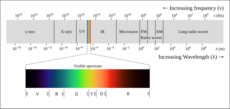
We often simplify complexity into discrete groups, but for most complex phenomena, I believe that it’s best to think of life as a spectrum. For example, while I look at my walls and say “they are blue”, a physicist who really understands color theory would be able to interpret the wavelength of light that is being reflected off these walls, and understands that that wavelength really just a point on an infinite spectrum (bound by a certain range).
Psychologists working in R often use numeric data, and see this as a list (or vector) of numbers. For example, below is data on the narcissism (variable = NPI; a measure of how self-absorbed; self-interested) of a group of Berkeley Haas MBA students were1.
1 These data come from the hormone_data.csv file, which should be updated to our course page. You’ll learn more about how to access these data files later in this chapter.
Professor Interpretation I learn a lot just from this simple output! 2
2 We’ll go over how to load datasets in R in Part 2. For this part of the chapter, the focus is on understanding what R is doing, and why we are doing it.
haas <- read.csv(“./chapter_data/hormone_data.csv”, stringsAsFactors = T”) is the R command that loads the dataset. Note that the path to the datafile - hormone_data.csv - is specific to the way I’ve stored these data in my file system. You’ll learn below how to change this to access your own dataset :)
haas$NPI is the R command that was used to generate the output below; a list of 122 individual Narcissism scores.
I know there’s 122 individual scores because R is keeping count for me using indexing; the numbers in brackets. [1] shows that the first person in the dataset has a narcissism (NPI) score of 3.43; [118] 3.73 shows that this is the score for the 118th person in the dataset, and then I can count up to 122. There are much faster ways to do this, but I can do it this way too :)
I also see there are a few missing data points in the responses - these are marked as NA. This could be people who didn’t complete the survey or were excluded for other reasons (e.g. missing data).
Graphing : The Histogram
Always always always graph your data. Graphs will help summarize, organize, and highlight important features of your data that would be impossible to see just by looking at numbers.3
3 yes, dear student, it is true : a picture is worth…a thousand words.
The Histogram is a common way researchers illustrate numeric variables. The histogram organizes data - you lose the individual values, but gain understanding in seeing how data are grouped together, which helps you observe patterns and get a quick summary of the variable.
There are two dimensions of a histogram :
the x-axis (the horizontal axis; what goes across) : displays the values of the variable as organized into groups (or “breaks”, in R).
the y-axis (the vertical axis; what goes up and down) : displays the frequency (or count) of the individuals in the data who “belong” to that group.
Let’s look at our MBA friends again, through the power of a histogram. As you look at a graph, it’s important to practice thinking about what you learn from the data. Let’s avoid fancy stats terminology for now; it’s not necessary for our purposes!!
hist(haas$NPI, xlab ="Narcissism Score", col ='black', bor ='white', main ="")
the code : this code draws a histogram using the hist() function. I’ve also added several arguments that change some of the default settings to give the graph some digital style.
xlab gives the x-axis of the graph a nice label.
colchanges the color of the bars to black.
bor changes the color of the lines surrounding the bars to white.
main changes the title. In this case, "" sets the title to be nothing, so there’s no title.
the graph : okay, what did R do!
x-axis : this reports the grouped values of the individual narcissism scores.
y-axis : this reports how many people were in each group.
professor interpretation with no fancy stats language needed.
most people (around 42?) had a narcissism score between 3 and 3.5
a few people were really high in narcissism…above a 4.5. I’m not sure from the graph exactly how many people were in this group, or what their score was.
a few people were really low in narcissism…below a 2. Again, I’m not sure from the graph exactly how many people were in this group, or what their score was, but I see their humble selves!
I also notice that this is not a super large study - the frequencies on the y-axis are relatively low numbers.
Activity : Think about Data!
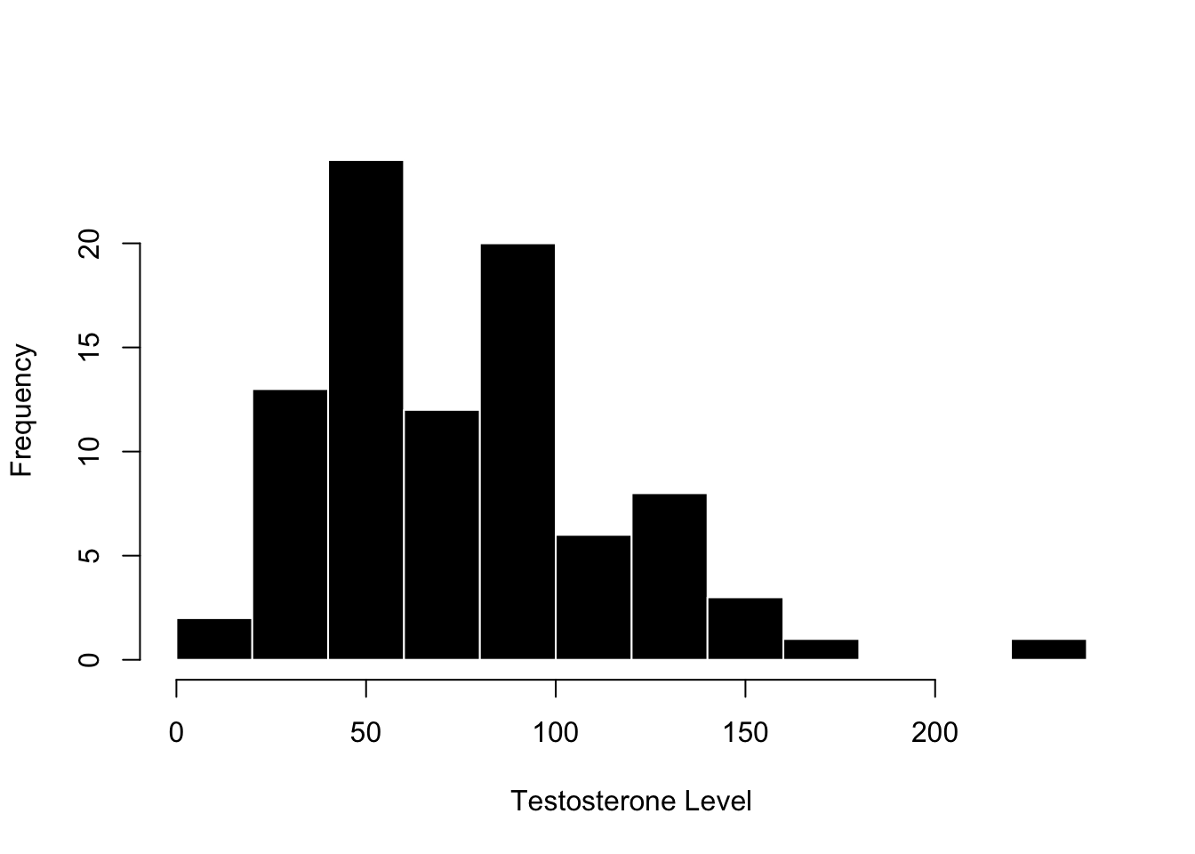
Okay, your turn. Below is a graph from the same MBA students, but this time measuring their testosterone levels. Look over the graph, THINK about what you see, and then expand the textbox below (click on the arrow on the right side of the green box) to see what I wrote.
hist(haas$test, xlab ="Testosterone Level", main ="", col ='black', bor ='white')
TipPROFESSOR SPOILERS : Expand this textbox when you are ready by clicking on the arrow —>
the graph
x-axis : this reports the grouped values of the individual testosterone scores, measured in some kind of density (pg/ML)
y-axis : this reports how many people were in each group.
what I see and observe with no stats language :
most people (around 25+12+20 = 77) had a testosterone level between 50 and 100.
there were no scores below zero (which makes sense) and one person who had a very high level of testosterone. I’m not a hormone researcher, but the non-negative values seems good, and I might want to make sure that there wasn’t some data entry error for the extreme score.
Again, I notice that this is not a super large study….and these relatively low numbers seem similar to the narcissism data, which makes sense since they came from the same study.
Categorical Variable
Definition : Categorical Variable
A categorical variable is when the values of the variable represent different groups (or categories). Categories are often useful and simple ways to group individuals together. For example, when I see a color, I don’t ever describe it in terms of its color hex code or specific wavelength - I just call it by the simple primary color that I got from the crayola box….maybe the 24 color version if I’m feeling fancy.
4 they are all one color - the human color. just kidding from the top left it’s 2, 3, 4, and 7. but I’m blue green color blind so you should argue with me in the comments.
The broad label for the variable is called the factor, and the specific groups of data are called levels. So in the color example, the category of color would be the factor, and the different groups of color would be the levels.
As another example, researchers can measure gender with categories such as female, male, transgender, and other. Identify the factor and levels in this example.
TipWhat are the factors and levels in the example above?
Factor : would be the variable of gender. Generally there’s one factor label for each variable.
Level : would be the categories female, male, transgender, and other.
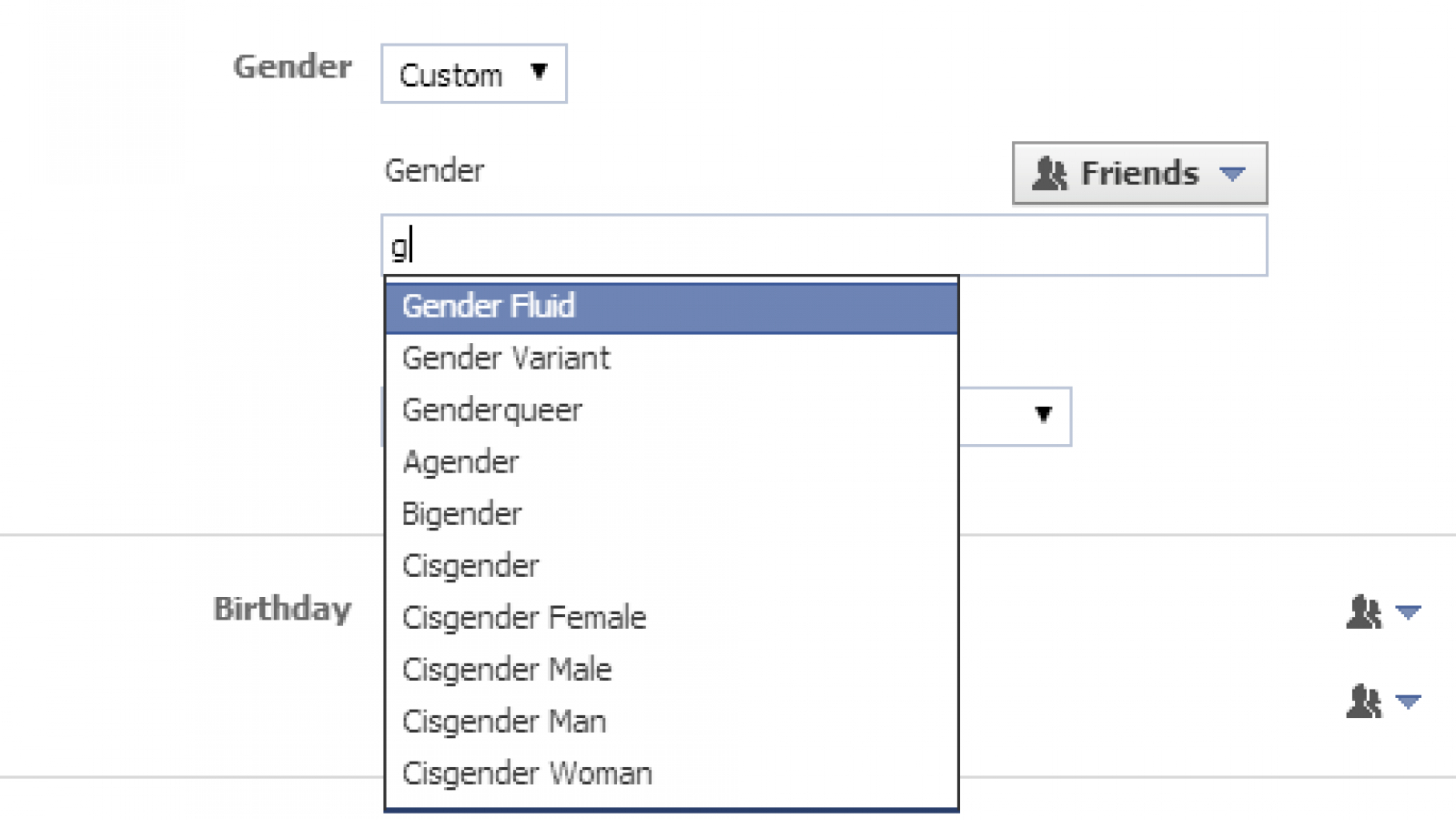
Culture in Statistics : Gender Identity
Hi folks! It’s me again, Open-Source Mickey Mouse to talk with you about the idea that statistics has a culture that is socially constructed by people like you!
One domain where this is particularly relevant is in the area of gender identity. While many people identify as “male” or “female”, some people don’t fit into these categories. (Seems pretty simple to me to let folks exist as they want! But I’m just a poor open-source servant freed from my corporate overlords.) Yet as folks in power have recently forced this narrow binary view of gender identity onto everyone, it becomes even more critical to engage with these ideas and try to define a science that can capture the complexity of human life in ways that let people be their full selves.
Unfortunately, most psychological researchers still hold on to Male / Female binaries in the way they measure gender or sex, yet there are many reasons - both scientific and humanistic - to give people more range to express important aspects of their identity.
Indeed, categories almost always oversimplify the complexity of life, yet are often used by people (and researchers) because they can sometimes be useful and simple shortcuts for us to understand the world.
If you are simply interested in doing a superficial survey of a variable like race, ethnicity, or gender, then I think categorical data can be a fine -if often unscientific - approach, and would recommend giving all people the chance to express their identity in some way. For example, here’s an article describing research on the way that exclusionary categories can negatively impact science, and offering clear and easy recommendations for reseachers to broaden science (e.g., reporting non-binary participants).
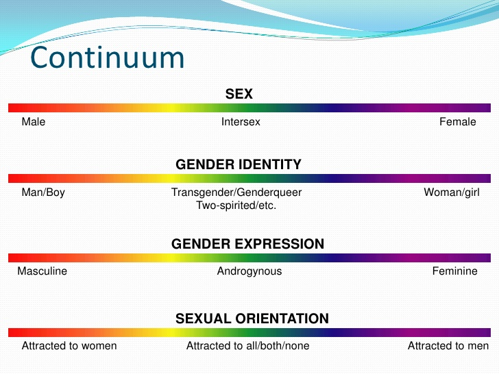
However, if you are interested in really digging into a variable, then a continuous approach is almost always best, since it allows for more flexibility in capturing complexity in variation. We’ll discuss more on how to do this in a few weeks when we learn about measuring continuous variables with likert scales.
5 a continuous approach to measuring gender. hi if u still reading, let me know if you have any thoughts on this section of the chapter.
Graphing : The Categorical Plot
The histogram only describes a graph for numeric data, since it organizes numbers into groups (it kind of turns complex variation into more simple categories). When the variable is categorical, people call it a plot 🤷.
This graph looks very similar to our histogram :
the x-axis (the horizontal axis; what goes across) : displays the levels of the factor variable.
the y-axis (the vertical axis; what goes up and down) : displays the frequency (or count) of the individuals in the data who “belong” to each group.
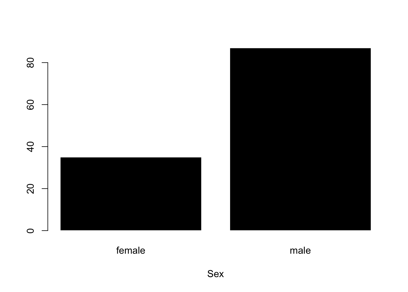
Alright, back to our good MBA friends. This is a graph of the categorical variable “sex”. Again, look over the graph, THINK about what you see (no stats terminology; what do you learn!), and then highlight my text to see what I wrote about.
plot(haas$sex, col ='black', bor ='white', xlab ="Sex")
The Code : this code draws a histogram using the plot() function. Note that I’ve asked R to plot the variable haas$sex. I’ve also added several arguments that change some of the default settings to give the graph some digital style.
xlab gives the x-axis of the graph a nice label.
colchanges the color of the bars to black.
bor changes the color of the lines surrounding the bars to white.
The Graph :
x-axis : this reports levels (female; male) of the categorical factor variable Sex.
y-axis : this reports how many people were in each group.
What I see and observe with no stats language :
It appears that the researchers only measured sex as a f/m binary (or that no participants reported a category other than female or male).
there were more males than females in this dataset. This matches my perception / stereotype of what a typical MBA program might look like; however I looked into it and Haas reports a larger percentage of female enrollments in the MBA program; so our data may not serve as a representative sample of the true population.6
6 Will learn about these ideas much later this semester! here’s a link to learn more about women in Haas. capitalism will eat us all eventually I guess, and good to challenge our stereotypes / perceptions!
Part 2 : Data and Datasets in R
The Dataframe
Definition : Rows and Columns
As a researcher, you’ll be interested in understanding not only one variable at a time, but will be interested in a dataset - multiple variables about an individual that are organized - in order to see how variables are related to each other (remember : this is a function of the linear model).
The datasets in our class will be stored on Dropbox; you can find a link to this on our course page, under the Course Materials module (see below for the image that you’re looking for).
You’ll learn how to load these datasets later in this lecture. For now, what is a dataset?
A dataset is really a dataframe - a two-dimensional way to organize data - and takes the following structure in this class.
the rows define the individual in the dataset. rows go across horizontally, like a rowboat going across a lake.
the columns define the variables in the dataset. go up and down vertically; like what might support a bridge.
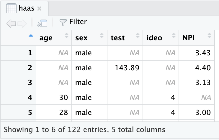
Look at the example below - again from our budding MBAs in the Haas program. What do you observe about the rows and columns? What does this tell you about the dataset?
In the example dataframe above - I see 5 rows (representing 5 individuals) and five columns (representing five variables like the person’s age, their sex, their testosterone levels, political ideology, and their NPI (Narcissism) score. or their Race, etc.) Note that the names of the variables do not count as a row, since these are not individuals in the dataset, and you would need to know more about the dataset to know that ideo = political ideology, or test = testosterone. I also see that R is helpfully telling me that this is only a snapshot of the entire dataset - the whole dataframe has 122 entries (rows), meaning that there’s 122 MBA students in this dataset, and 5 total columns (which we can all see here.)
As a researcher, you have access to an entire dataset (either collected by you or another researcher) that organizes multiple variables for each individual. This semester, we’ll work with a variety of datasets on different psychological topics - not just haas students.
Definition : Indexing
The dataset gives us access to all the individual rows and columns at once, we will often want to focus on one specific variable (or individual) at a time. Indexing refers to a flexible method of selecting a specific set of data from a larger collection. Previously’ we’ve seen indexing when asking R to produce a large set of numbers; for example asking it to count from 1 to 100.
The indexing shows up as brackets next to the actual data, and is way for R to index that the [1]st data entry is the number 1, the [24]th entry is the number 24, and so on.
When I ask R to show me the dataset haas, the output can be overwhelming. Below is what R shows you when you ask to see the haas dataset. And this is a relatively small dataset with just 122 individuals (rows) and five variables (columns).
haas
    age    sex   test ideo  NPI
1    NA   male     NA   NA 3.43
2    NA   male 143.89   NA 4.40
3    NA   male     NA   NA 3.13
4    30   male     NA    4   NA
5    28   male     NA    4 3.00
6    33 female     NA    5   NA
7    NA   male     NA   NA 3.05
8    NA   male     NA   NA   NA
9    NA   male  77.95   NA   NA
10   NA   male     NA   NA 3.63
11   26   male 126.29    3 3.95
12   31   male  59.48    5 3.08
13   27   male  89.45    4 3.83
14   27   male  82.80    3 3.23
15   28   male  97.39    4 3.80
16   30   male  54.80    4 1.80
17   28   male  46.07    4 3.68
18   24   male     NA    4 3.48
19   32   male  87.40    3 2.73
20   25   male  85.01    4 3.40
21   27   male     NA    3 2.95
22   25   male     NA    4 3.65
23   24   male 102.86    3 2.88
24   28   male  73.60    3 2.50
25   27   male     NA    2 3.13
26   29   male  90.68    4 2.75
27   28   male  44.70    3 3.00
28   29   male     NA    4 3.15
29   30   male  77.61    4 3.30
30   26   male  57.20    5 3.20
31   31   male  49.92    4 2.43
32   28   male     NA    3 3.13
33   32   male     NA    5   NA
34   27   male  85.01    2 3.33
35   32   male  74.86    2 2.88
36   27   male 125.89    3 2.55
37   29   male  77.07    4 3.35
38   30   male     NA    4 3.30
39   26   male  30.54    4 3.28
40   27   male  73.76    3 3.08
41   32   male  65.61    3 2.48
42   29   male  51.23    4 2.78
43   28   male  85.17    3 4.58
44   28   male     NA    3 2.53
45   29   male  57.14    2 2.78
46   30   male  65.31    4 2.88
47   28   male  53.07    4   NA
48   28   male 104.65    3 3.43
49   31   male  90.32    3 2.48
50   NA female  24.71   NA 3.50
51   26 female  20.99    3 2.40
52   27 female     NA    4 3.28
53   28 female     NA    3 3.63
54   28 female   5.51    5 3.13
55   27 female  40.49    4 2.05
56   25 female  35.05    2 2.98
57   26 female  57.71    4 2.53
58   26 female  27.36    4 3.45
59   27 female  59.37    3 2.80
60   26 female  21.63    3 2.60
61   29 female     NA    3 2.05
62   25 female     NA    7 2.60
63   37 female  39.50    4 2.73
64   28 female  42.35    4 3.25
65   24 female  32.42    3 2.78
66   29   male  97.63    4 2.93
67   28   male 131.51    3 3.08
68   26   male     NA    4 3.33
69   27   male     NA    5 4.05
70   29   male     NA    2 3.65
71   27   male 140.53    2 3.15
72   26   male     NA    3 3.33
73   28   male     NA    3 3.98
74   22   male  90.88    5 4.48
75   29   male 148.24    5 3.00
76   29   male 132.24    4 3.00
77   27   male  82.43    4 3.25
78   26   male  73.43    4 4.28
79   35   male     NA    2 3.13
80   27   male 100.49    4 3.83
81   25   male  94.31    4 3.98
82   27   male  72.53    2 4.13
83   30   male 133.35    4 3.73
84   27   male  59.77    4 3.28
85   30   male  91.83    4 2.85
86   29   male  82.13    3 3.28
87   30   male 172.15    3 3.70
88   29   male 228.17    2 3.03
89   27   male 133.70    3 3.38
90   27   male  89.24    4 2.88
91   28   male  88.62    3 3.20
92   28   male  86.83    4 3.40
93   25   male 138.65    4 3.70
94   33   male  59.75    4 3.50
95   28   male  46.30    3 2.58
96   31   male 107.02    3 2.90
97   24   male  60.16    2 3.00
98   26   male     NA    4 3.35
99   27   male 107.71    3 2.63
100  23   male  99.64    2   NA
101  32   male 131.51    3   NA
102  29   male  91.94    4 4.05
103  25   male  53.67    3 3.43
104  25   male     NA    4 4.28
105  27 female     NA    4 3.00
106  27 female  59.24    2 3.10
107  30 female  28.03    5 3.13
108  28 female  33.38    5 2.83
109  26 female  53.31    4 2.78
110  28 female  27.53    4 2.33
111  29 female  16.89    4 2.68
112  25 female  51.53    4 2.88
113  26 female  37.15    4 2.53
114  27 female  50.55    2 3.80
115  28 female     NA    4 3.48
116  28 female  41.35    5 3.15
117  29 female  64.66    5 4.38
118  24 female  37.95    2 3.73
119  27 female  54.26    4 3.80
120  27 female     NA    4 2.60
121  27 female 113.41    4 3.38
122  29 female  41.35    3 3.13
I am overwhelmed with data. So it will be important to find ways to target the data that we want. There are several ways we can do this!
Because a dataset has two different dimensions, we have to use two coordinates to index the dataset - one coordinate for the row(s) that we want to focus on, and one coordinate for the column(s) that we want to focus on.
Indexing an Entire Dataset
Because a dataset has two different dimensions, we have to use two coordinates to index the dataset - one coordinate for the row(s) that we want to focus on, and one coordinate for the column(s) that we want to focus on.
data # this reports the entire dataset. In the example to the right, I’ve typed in haas (since this is the name of the dataset in this example) and see the dataset reported.
data[i, j] # this code returns a specific row (i), and a specific column (j). The convention is to use the letter i for a row first, then j for a column [you can remember this order as RC Car, or R is Cool]. For example
haas[2,3]
[1] 143.89
Shows me that R has highlighted the second row and third column of the dataset - the second person’s testosterone level is 143.89 units.
data[ , j] # if you leave a blank for the rows, then R will return all of the rows, and whatever column you specify. This can be good for looking at a specific variable for all individuals. For example, the following code returns all of the testosterone data (the third column).
```{r}haas[,3]```
data[i, ] # if you leave a blank for the column, then you would see all of the columns for a specific row. This can be good for looking at a specific individual’s entire dataset; such as all of participant 2’s data below.
haas[2,]
  age  sex   test ideo NPI
2  NA male 143.89   NA 4.4
haas[i:i, c(j, j)] # you can adapt this code to give a range of values too. for example, if I want to see rows 4-10 and columns 1 and 3, I would run the following code.
haas[4:10, c(1,3)]
   age  test
4   30    NA
5   28    NA
6   33    NA
7   NA    NA
8   NA    NA
9   NA 77.95
10  NA    NA
Indexing a Single Variable
data$variable # You can also use the $ (dollar sign) in R to reference a single variable from a dataset. This is very useful, because you can use the name of the variable instead of the numerical index. So, for example, if I want to highlight the testosterone levels of the haas dataset, I would run the following :
haas$test
  [1]     NA 143.89     NA     NA     NA     NA     NA     NA  77.95     NA
 [11] 126.29  59.48  89.45  82.80  97.39  54.80  46.07     NA  87.40  85.01
 [21]     NA     NA 102.86  73.60     NA  90.68  44.70     NA  77.61  57.20
 [31]  49.92     NA     NA  85.01  74.86 125.89  77.07     NA  30.54  73.76
 [41]  65.61  51.23  85.17     NA  57.14  65.31  53.07 104.65  90.32  24.71
 [51]  20.99     NA     NA   5.51  40.49  35.05  57.71  27.36  59.37  21.63
 [61]     NA     NA  39.50  42.35  32.42  97.63 131.51     NA     NA     NA
 [71] 140.53     NA     NA  90.88 148.24 132.24  82.43  73.43     NA 100.49
 [81]  94.31  72.53 133.35  59.77  91.83  82.13 172.15 228.17 133.70  89.24
 [91]  88.62  86.83 138.65  59.75  46.30 107.02  60.16     NA 107.71  99.64
[101] 131.51  91.94  53.67     NA     NA  59.24  28.03  33.38  53.31  27.53
[111]  16.89  51.53  37.15  50.55     NA  41.35  64.66  37.95  54.26     NA
[121] 113.41  41.35
data$variable[i] # We can then use indexing to narrow this down. Because a variable only has one dimension (it’s just a collection of individuals; not rows and individuals) I only need to use one coordinate to index the specific individual(s) I want to find.
haas$test[2]
[1] 143.89
data$variable[i:i] # Can be used to find a range of individuals. These numbers need to be sequential for this code to work.
haas$test[1:3]
[1] NA 143.89 NA
data$variable[c(i,i,i)] # If you want to find individuals who are not next to each other, you need to use the c (combine) function to combine multiple coordinates together. You can have as many coordinates here as you want. For example :
haas$test[c(2,3,14:18, 116:118)]
[1] 143.89 NA 82.80 97.39 54.80 46.07 NA 41.35 64.66 37.95
Test Yourself : Indexing!
Okay, practice time. Use the haas dataset and your knowledge of indexing to identify what R would show if you typed in the following commands (no R required)
haas$age[47]
haas$NPI[1:3]
haas[51,2]
haas[60, ]
haas[ , 6]
TipAnswer Key : Indexing!
28
3.43 4.40 3.13
female
26 female 21.63 3 2.6
you would get an error; there is no 6th column.
In R : How to Navigate Datasets
Let’s get some more practice with some actual data. Before we learn how to import data in R, we can work with a super exciting dataset that is already part of the R program - a dataset on the weights of chickens (chkwt).
Watch the two videos below to see how I navigate this dataset; here’s a link to the RScript that I use in the videos.
Video : Checking Datasets in R
length() : counts the number of objects (variables) in a dataset (or any object)
nrow() : counts the number of rows (participants) in a dataset
head() : looks at the first six rows of a dataset
Video : Navigating Datasets with Indexing
Use this video to answer the check-in questions below.
Use the fake dataset below and your knowledge of navigating datasets with indexing to identify what answer R would give if you gave it the following code. (Note : no R is needed to complete this problem).
As a researcher, you will work with data that you (or other researcher friends) have collected. The .csv file (csv stands for comma separated variables) is one of the most common formats for storing data that you will encounter. You’ve probably encountered this before, and likely have opened this file type in a program like excel or google sheets. But in this class, we’ll learn to load these files directly into R. Using R has two advantages :
R is way more powerful than excel or Google Sheets.
R allows us to document all of our steps. This semester, we’ll learn how to make changes to the dataset (e.g., changing the names of a variable; removing bad data; transforming data). It’s important to be completely transparent about these changes, and doing these changes in R (with an R Script!) will ensure that we document our steps for our future selves / other researchers.
Videos : How to Load Datasets in R
There are two different ways to load a data file into R : one way (“the point and click method”) involves clicking some boxes, like most of y’all are used to doing. The second way involves typing in an R command. Below are videos that highlight each method.
Important
Regardless of which method you use, there are three things you want to check every time you load data : change the name of the dataset (to make it something simple to type and memorable); check the headers (make sure the variables have names, since sometimes), and set stringAsFactors = TRUE (which will automatically convert all your string variables into categorical factor variables, which is almost always what you will want to do in this class.
These instructions are highlighted because students often forget. So note the importance! They are important steps!!!
Video : Importing Data with the “Point and Click” Method and Console Method
the “point and click” method of loading data
the console / Rscript method of loading data
Video : For Posit Users : working with projects and loading data in the cloud.
posit.cloud users! You will need an extra step that folks using posit.cloud have to use to upload datasets to the cloud (and then import them).
Practice Quiz 2
Okay, this was a LOT. Like drinking water from a fire hose. I promise this will get easier, and it just requires practice. Let’s see how clear the professor’s instructions were with this…practice quiz!
Here’s a video key with the practice quiz answers. Please attempt the quiz on your own; if you get stuck, refer to the relevant videos above. And feel free to reach out on Discord if something’s confusing or I got something wrong. Appreciate y’alls engagement!
Part 3 : Research for Fun and Profit
Researchers share their knowledge with others in scientific articles. These are written by researchers for other researchers, tend to be very detailed and technical, and are a researcher’s golden ticket to getting a job, research grant, invited talk or book deal, podcast invitation, etc. So there’s a lot of pressure to publish research among academics.
The Publication Process
Researchers spread their scientific knowledge by publishing research papers. You can read more about how researchers publish research HERE. However, the TLDR is something like this :
Researcher has an idea! They assemble a team of others interested in the idea, and do a literature review in order to gain background knowledge on the topic.
Researcher designs a study, collects data, analyzes the data, and writes up the data as a report. All the steps of the scientific method. This is what you will do for the final project!
Researcher submits the report to a scientific journal. A journal is a collection of articles that are usually united by some common theme. In general, the shorter the name of the journal, the more prestigious7. For example, the “Journal of Research in Personality” is considered less prestigious than the “Journal of Personality and Social Psychology”, which is less prestigious than the journal called “Psychological Science”, which is considered less prestigious than the journal called “Science”.
An editor decides whether to review or reject the article. Editors make an initial decision - based on a summary of the study and a letter that the author writes to the editor - whether the research article might be a good fit for the journal. If so, they pass it along to the next step. If not, they send a “Thanks, but….” rejection letter.
The editor sends the article to peer-reviewers. Peer reviewers are other researchers who have some related research interests or skills in the topic of the paper. They will look over the article. The editor may know these people, or they get asked by another peer-reviewer who didn’t want to do it but nominated someone else to step into the role. Peer-reviewers work on a completely voluntary basis - it’s seen as required service, and there’s a bit of professional reputation to maintain in doing this work. Yes, there are problems with unpaid labor in academia. We can chat about that if you’d like; ask questions / raise it as an issue on Discord.
The editor makes a decision on the paper based on the feedback from the peer-reviewers. The editor summarizes the feedback, and either accepts the paper, accepts as long as the person makes necessary revisions, asks the researcher to “Revise and Resubmit” (this is called an R&R - probably the most common outcome, and does not guarantee that the paper will be accepted if the revisions are made, but will get sent out to peer-reviewers again), or rejects the paper. In any case, the author will see the comments made by the peer-reviewers and the editor.
The (accepted) paper goes to a proofreader and is published. Hooray! This process probably takes anywhere from 6 months (insanely fast) to 2 years (or more, depending on the number of revisions that are required).
7 Prestige is a very subjective concept in science. However, scientists have found many ways to quantify it, as described in the sections below!
Publish! Or Perish…?
Ask any grad student or professor - the publication process is stressful, unpredictable, slow, and threatening. Grad students are required to publish papers in order to have a chance at an academic job as a researcher (and even extremely productive and thoughtful graduate students are not guaranteed an academic job), professors are required to publish papers in order to get a chance of getting tenure (and even extremely productive and thoughtful researchers are not guaranteed tenure).
This creates incredible pressure on researchers to get results; pressure that often can interfere with people’s ability to do GOOD science. We’ll talk about this more throughout the semester; bring questions to class / Discord!
Types of Research Articles
We’ll learn how to read and dissect scientific articles this semester, but first it will be important to learn how to identify the different types of articles. There are a few different types of articles that researchers write :
Original Reports : An original report is where the researcher(s) write about the results of a novel study they did to test some theory. This means the researchers did something “new” - usually they collected and analyzed new data to test a theory, or analyzed existing data in a new way. Here’s an example of an original report on the topic of emotion regulation.
Replication : A replication is a type of study where a researcher repeats the steps they (or another) researcher did, and sees if they get the same result. As we discussed, psychology (and many other fields) is in a replication crisis. This type of article was not very common before the 2010s, but is more common now. Still, faculty tend to be biased toward producing original reports - a school like Berkeley or Stanford would not hire a researcher just for doing replications. Here’s an example of a replication on the topic of emotion regulation. Note this is not really a direct replication, since they replicated in a different population.
Meta-Analyses : A meta-analysis is where researchers take other people’s data, collect it, and analyze it in order to see broad trends across an entire field. For example, a meta-analysis might take all the research on whether there’s a relationship between playing violent video games and violent behavior, and analyze this existing research in terms of common themes, such as the type of video games the researchers studied, the measures of violence, and the results. Meta-Analyses can be a great way to look at a broad trend, but they rely on the assumption that the individual studies they summarize are, in fact, valid themselves. That is, if there are systematic biases in the way researchers study a topic, the Meta Analysis won’t solve or even identify those problems. Here’s an example of a meta-analysis done on the topic of emotion regulation.
Review Article : Review articles summarize existing research without doing any additional data analysis (in contrast to a Meta-Analysis, in which there is data analysis of past research). This is the closest thing to a paper you might write in an English class - the authors take past research, summarize it in terms of common themes, and maybe highlight limitations, or new directions the field might take. Review articles are a great way to get a broad overview of a topic, since they summarize and organize past research, and will often highlight next steps that researchers should take. Here’s an example of a review article done on the topic of emotion regulation.
The Peer Review Process
In order to publish their results, researchers have their peers review their work, and provide comments or suggestions. The peer-review process ideally serves two purposes :
Peer Reviewers Help Improve the Research. The peers doing the reviewing are supposed to have expertise in the topic of the paper. This allows them to suggest ways to improve the paper. These suggestions can run from the simple (such as recommending other researchers to reference in the introduction or additional analyses to run) to very involved (suggestions for additional studies to run, different methods to use, or different people to study).
Peer Reviewers Provide a Vote of Confidence in the Ideas and Analyses of the Paper. The editor of a journal will look to the peer reviewers for evidence that the research is “high quality” and / or novel enough to be published. There’s a fair amount of bias here - some reviewers think the research is good but not considered a “good fit” for the journal. But the “peer-reviewed” label of a journal gives at least one layer of confidence that some other people like this research.
One important aspect of the peer-review process is that the peer-reviewers are anonymous to the author, and sometimes the author is anonymous to the peer-reviewers. Ideally, this helps prevent previous beliefs bias (since some researchers may have positive or negative impressions of each other) and social influence bias (since a famous researcher at a fancy school may have their research more trusted than someone with less prestige to their name or institution). However, psychological fields are often small enough that people tend to know who’s doing what research, and there are other cues that can tip peer-reviewers off about who the author of a study is (for example, the author of a study will likely reference their own work, since their new study builds off their old study.)
WarningAcademic Publishers are Predatory Capitalists.
You know how the music business can hurt artists and interrupt the free flow of groovy music??? Well, academic publishers are no different, and can make profits in the billions of dollars. They do this by charging exorbitant fees for accessing peer-reviewed articles, and not paying the researchers who publish papers any money. That’s right; researchers get a 0% commission of any sales of their academic articles. It is a horrible and corrupt system that deserves to die.
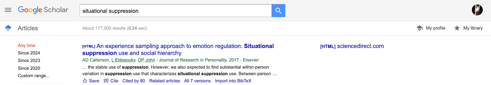
Next week we will find research articles related to YOUR research interests. I like to use Google Scholar for this - I find the search features powerful and Google will comb the internet for free versions of research articles (so I don’t have to be on campus or have proxy access to a college library, or “steal” articles from predatory publishers who don’t pay authors using tools like sci-hub or annas-archive).
For example, searching for one of my dissertation chapters shows this page.
How to Find Articles
Some tips for finding an article related to your topic :
Use the right “jargon”. As part of the operationalization process, scientists use specialized terms. What you might call “holding it in” researchers call “expressive suppression”; a “jerk” would be someone “low in agreeableness”; that feeling of “being hella stressed before an exam but also low key stepping up because of that stress” is the “psychophysiological distinction between challenge and threat”. As you search for research related to your topic, take note of how researchers are describing related phenomena, and adjust your terms as needed. This is part of building your schema for the topic.
Look at past research on the topic. If you’ve found a relevant article on your topic, it’s likely that the article has referenced other research that is also relevant. Read or scan through the introduction (or the references section) and see if there’s something that looks related to your interests.
Look at future research on the topic. If you found a relevant article on your topic, it’s likely that other researchers have also read that article, and used it in their future research. Google Scholar has a “Cited By” button []that you can use in order to see more recent articles that have referenced the article you found. This is a particularly useful way to find more recent research if you found a “classic” in the field, or check for replications or controversies.
Old Research is Okay! But look for new research too. Many students wonder if an “old” study is still relevant. Some papers are “classics” in the field, and great to read. But it’s likely that our field’s understanding of self-esteem has changed from 1970. If you are hoping to build your schema on a topic, finding a review article from the last 10 years (or 5; or 2!) would be a good place to start.
How to Evaluate an Article
It can often be overwhelming for students to sift through the masses of research on a topic and know what’s most important and relevant.
Reading the article and using your critical thinking skills / psychological training is the best approach. To do this, it is recommended to go to Graduate School, where you can spend multiple years reading as much as you want on a beautiful college campus, taking classes where you can deeply engage with the research and ideas, immerse yourself in meaningful intellectual conversations had by other graduate students and kindly professors - the gleam of knowledge and excitement of supporting the next generation of researcher in their eye. Oh, that is not interesting to you / grad schools are flooded with applications / you can’t get an office hour appointment with your professor who actually / you don’t have the privilege of spending 5-8 years getting paid near-poverty wages to be a poor scholar?
Well, below are a few other ideas to make superficial, all depending on our good friend social influence bias :
The Citation Count. Google scholar allows you to see how many other research articles have referenced the article that you found. While this can be a nice way to see how influential a paper is, a paper could be referenced a lot for reasons other than its validity, and maybe no one has read the most amazing paper in the world.
The Impact Factor of the Journal. Journals have different “prestige factors”, and the impact factor is one way to quantify this prestige. Impact factor is usually defined as the number of times the average article in a journal has been referenced by other researchers in a year. So an impact factor of 2 means that each article in that journal is referenced by two other articles in a year. The impact factor is something you have to look up - journals usually track this. I wouldn’t spend too much time worrying about it, but it’s a quick way to get a very superficial sense of the journal’s reputation. For example, let’s see how the impact factor relates to our rule of “broader journal name = more prestige”.
Journal
Impact Factor According to Google in 2024
Journal of Research in Personality
2.6
Journal of Personality and Social Psychology
6.4
Psychological Science
10.1 [couldn’t find a recent stat on this tho]
Science
44.7 [this escalated quickly]
The Researcher and Institution. Another way to evaluate an article is by evaluating the author. Does it look like this research has produced other cool research, or do you find their work boring and problematic for some reason? Is this researcher well known and respected in the field? Do they seem to have a happy photo with all their graduate students on their lab website, or is their lab website 10 years old and just has one sad looking graduate student asking for help with their eyes? Has the researcher continued to produce interesting, reliable research? Or were they the subject of a replication scandal?
Video Examples : Using Google Scholar to Find Research
Using Google Scholar
How to find articles, use the right jargon, and do some very superficial evaluations of the article’s quality.
Exporting APA Citations
The “” button on Google Scholar makes life so much easier!! No more memorizing APA format!! Hooray!!!
TLDR
We learned about different kinds of data (numeric and categorical), and how to graph and interpret these data. We also learned how to load and navigate datasets in R in order to look at variables.
In class this week, we will continue to get practice working with datasets and variables. Yeah!