Lecture 9 - Multiple Regression

Check-In : Testing Theories

Use the R output below to answer the questions in the check-in.

Model 1 : Predicting Handwashing from Gender

mod1 <- lm(Handwash ~ gender, data = d)
summary(mod1)

Call:
lm(formula = Handwash ~ gender, data = d)

Residuals:
    Min      1Q  Median      3Q     Max 
-3.5659 -0.5659  0.4341  0.7437  0.7437 

Coefficients:
            Estimate Std. Error t value Pr(>|t|)    
(Intercept)  3.25628    0.06065  53.688  < 2e-16 ***
genderW      0.30957    0.08515   3.636 0.000313 ***
---
Signif. codes:  0 '***' 0.001 '**' 0.01 '*' 0.05 '.' 0.1 ' ' 1

Residual standard error: 0.8556 on 402 degrees of freedom
  (438 observations deleted due to missingness)
Multiple R-squared:  0.03184,   Adjusted R-squared:  0.02943 
F-statistic: 13.22 on 1 and 402 DF,  p-value: 0.0003131

plotmeans(Handwash ~ gender, data = d,
          col = "white", barcol = "white", ylim = c(1,5))

Agenda & Announcements

1. Brain Exam is THIS WEEK in Discussion Section
   • start discussion section with a review / practice
   • then the brain exam : 12 minutes.
2. Milestone #5 : Due Monday.
3. Milestone #6 : Nah.
4. THE END IS NEAR
   • NEXT WEEK : Project Workshop
   • LAST CLASS : The learning has stopped. So what did we learn again?
   • RRR Week (Virtual) Project Workshop…basically professor office hours for whoever shows up.
5. TODAY :
   • 3:10 - 4:00. NHST and Brain Exam 2 Review
   • 4:00 - 4:30. Multiple Regression (More Regression)
   • 4:30 - 4:40. Break Time.
   • 4:40 - 5:00. More Multiple Regression
   • 5:00 - 6:00. Project Workshop Time (Milestone 4 Review)

Check-In Review : NHST Practice

Other Questions About Model 1.

1. What are the four reasons we might observe this pattern?
2. How might sampling bias influence these results?
3. How might measurment error influence these results?

More Practice? For the models below.

1. What’s the relationship between the two variables?
2. Is this relationship considered “statistically significant”? Why / why not?
3. Is this relationship considered “large”? Why / why not?
4. Critical Thinking :

Model 2 : Predicting Handwashing from Conscientiousness (Personality)

mod2 <- lm(Handwash ~ CONSC, data = d)
summary(mod2)

Call:
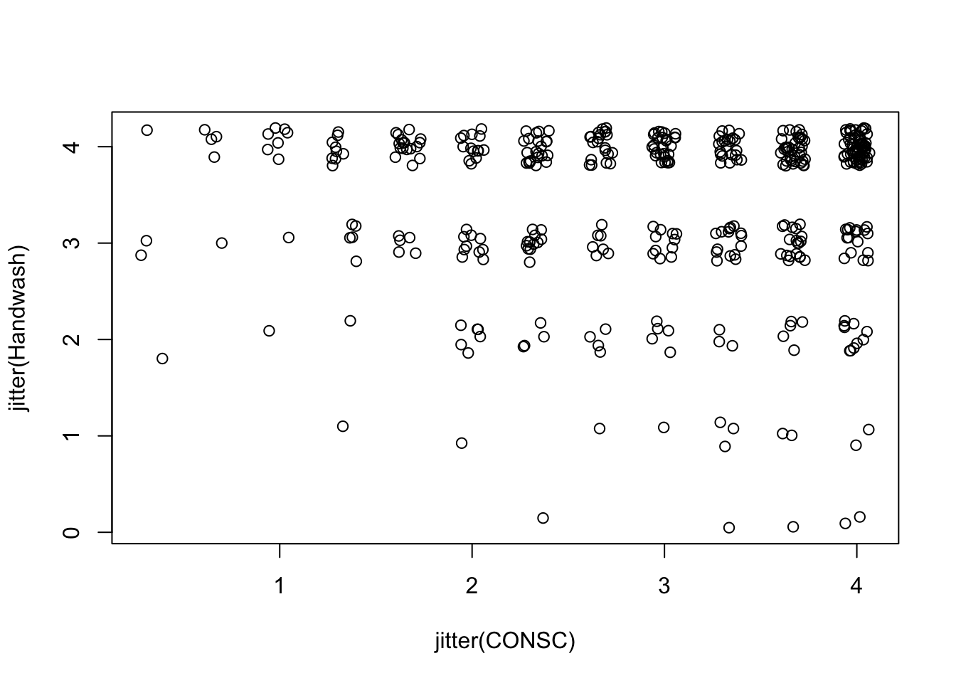
lm(formula = Handwash ~ CONSC, data = d)

Residuals:
    Min      1Q  Median      3Q     Max 
-3.4263 -0.4142  0.5677  0.5919  0.6039 

Coefficients:
            Estimate Std. Error t value Pr(>|t|)    
(Intercept)  3.46854    0.14382  24.117   <2e-16 ***
CONSC       -0.01812    0.04628  -0.392    0.696    
---
Signif. codes:  0 '***' 0.001 '**' 0.01 '*' 0.05 '.' 0.1 ' ' 1

Residual standard error: 0.8688 on 403 degrees of freedom
  (437 observations deleted due to missingness)
Multiple R-squared:  0.0003804, Adjusted R-squared:  -0.0021 
F-statistic: 0.1534 on 1 and 403 DF,  p-value: 0.6956

plot(jitter(Handwash) ~ jitter(CONSC), data = d)

Model 3 : Predicting Handwashing from Political Orientation

mod3 <- lm(Handwash ~ political_party, data = d)
summary(mod3)

Call:
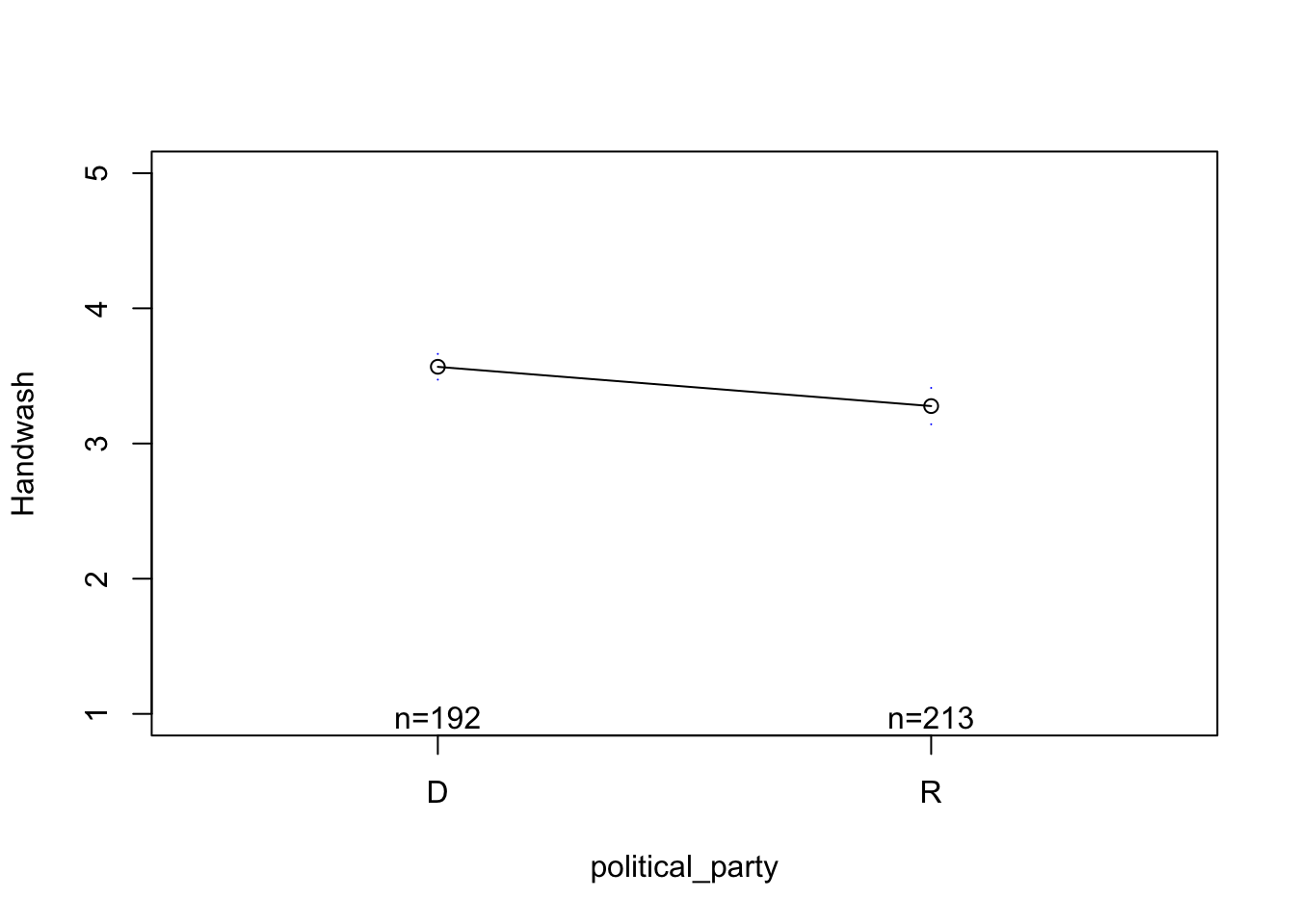
lm(formula = Handwash ~ political_party, data = d)

Residuals:
    Min      1Q  Median      3Q     Max 
-3.2770 -0.5677  0.4323  0.7230  0.7230 

Coefficients:
                 Estimate Std. Error t value Pr(>|t|)    
(Intercept)       3.56771    0.06183   57.70  < 2e-16 ***
political_partyR -0.29071    0.08525   -3.41 0.000715 ***
---
Signif. codes:  0 '***' 0.001 '**' 0.01 '*' 0.05 '.' 0.1 ' ' 1

Residual standard error: 0.8567 on 403 degrees of freedom
  (437 observations deleted due to missingness)
Multiple R-squared:  0.02804,   Adjusted R-squared:  0.02563 
F-statistic: 11.63 on 1 and 403 DF,  p-value: 0.0007153

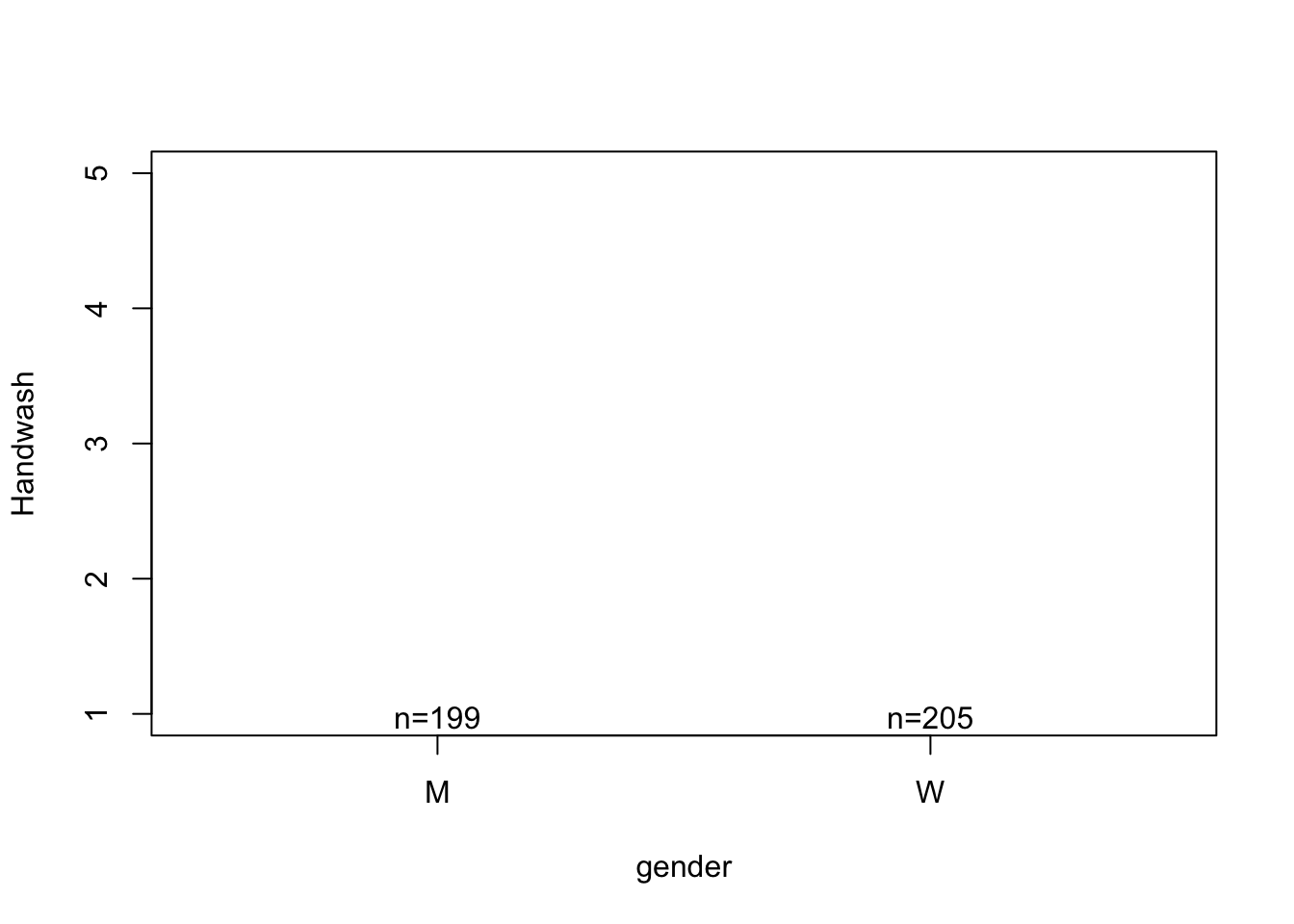
plotmeans(Handwash ~ political_party, data = d, ylim = c(1,5))

Warning in arrows(x, li, x, pmax(y - gap, li), col = barcol, lwd = lwd, :
zero-length arrow is of indeterminate angle and so skipped
Warning in arrows(x, li, x, pmax(y - gap, li), col = barcol, lwd = lwd, :
zero-length arrow is of indeterminate angle and so skipped

Warning in arrows(x, ui, x, pmin(y + gap, ui), col = barcol, lwd = lwd, :
zero-length arrow is of indeterminate angle and so skipped
Warning in arrows(x, ui, x, pmin(y + gap, ui), col = barcol, lwd = lwd, :
zero-length arrow is of indeterminate angle and so skipped

Some Pre-Recorded NHST Review Videos

• Note : I used last semester’s dataset for these examples, so you will likely get different results if you try and replicate in this semester’s class; a good example of how NHST doesn’t really tell us whether the results are “truth” or not, or whether they will replicate, etc.

• Example 1 : LOVEWATER ~ smoke.pot

• Examples 2 - 4 : faster explanations!

Chapter 10 Recap : Multiple Regression (Hair Length Predicts Height?!?!?????)

Data Cleaning and Descriptive Statistics

## Data Cleaning
library(gplots)
d <- read.csv("~/Dropbox/!WHY STATS/Class Datasets/101 - Class Datasets - FA25/mini_cal_data.csv", stringsAsFactors = T)

d$height[d$height < 10 | d$height > 100] <- NA
levels(d$is.female)[1] <- NA
#levels(d$long.hair)[1] <- NA

par(mfrow = c(1,3))
hist(d$height)
plot(d$is.female, xlab = "Is Female?")
plot(d$long.hair, xlab = "Has Long Hair?")

Activity and Discussion : Comparing Models

1. ICE-BREAKER :

   1. let’s keep it light mode : if you HAD to get a tattoo, what would you get? where would you get it? would it face toward you or other people?

   2. bring on the heavy mode : if you could change one thing about your childhood, what would you change?

2. MODEL INTERPRETATION : What Do You Observe in Model 1? Model 2?

3. MODEL 3 : What Do You Observe Changing About the Slopes from the Bivariate Model (Models 1 and Model 2) to the Multivariate Model (Model 3)?

4. Other Questions That You, the Students, Have?

Height ~ long.hair

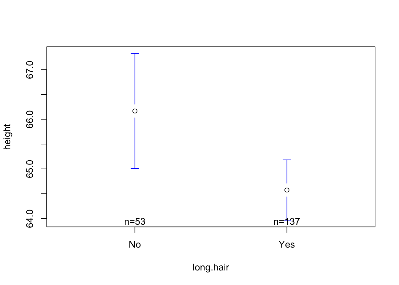
moda <- lm(height ~ long.hair, data = d)
summary(moda)

Call:
lm(formula = height ~ long.hair, data = d)

Residuals:
     Min       1Q   Median       3Q      Max 
-13.1660  -2.5734  -0.5734   2.4266  10.4266 

Coefficients:
             Estimate Std. Error t value Pr(>|t|)    
(Intercept)   66.1660     0.5187 127.568  < 2e-16 ***
long.hairYes  -1.5927     0.6108  -2.607  0.00985 ** 
---
Signif. codes:  0 '***' 0.001 '**' 0.01 '*' 0.05 '.' 0.1 ' ' 1

Residual standard error: 3.776 on 188 degrees of freedom
  (9 observations deleted due to missingness)
Multiple R-squared:  0.0349,    Adjusted R-squared:  0.02977 
F-statistic: 6.799 on 1 and 188 DF,  p-value: 0.009854

plotmeans(height ~ long.hair, data = d, connect = F)

Height ~ is.female

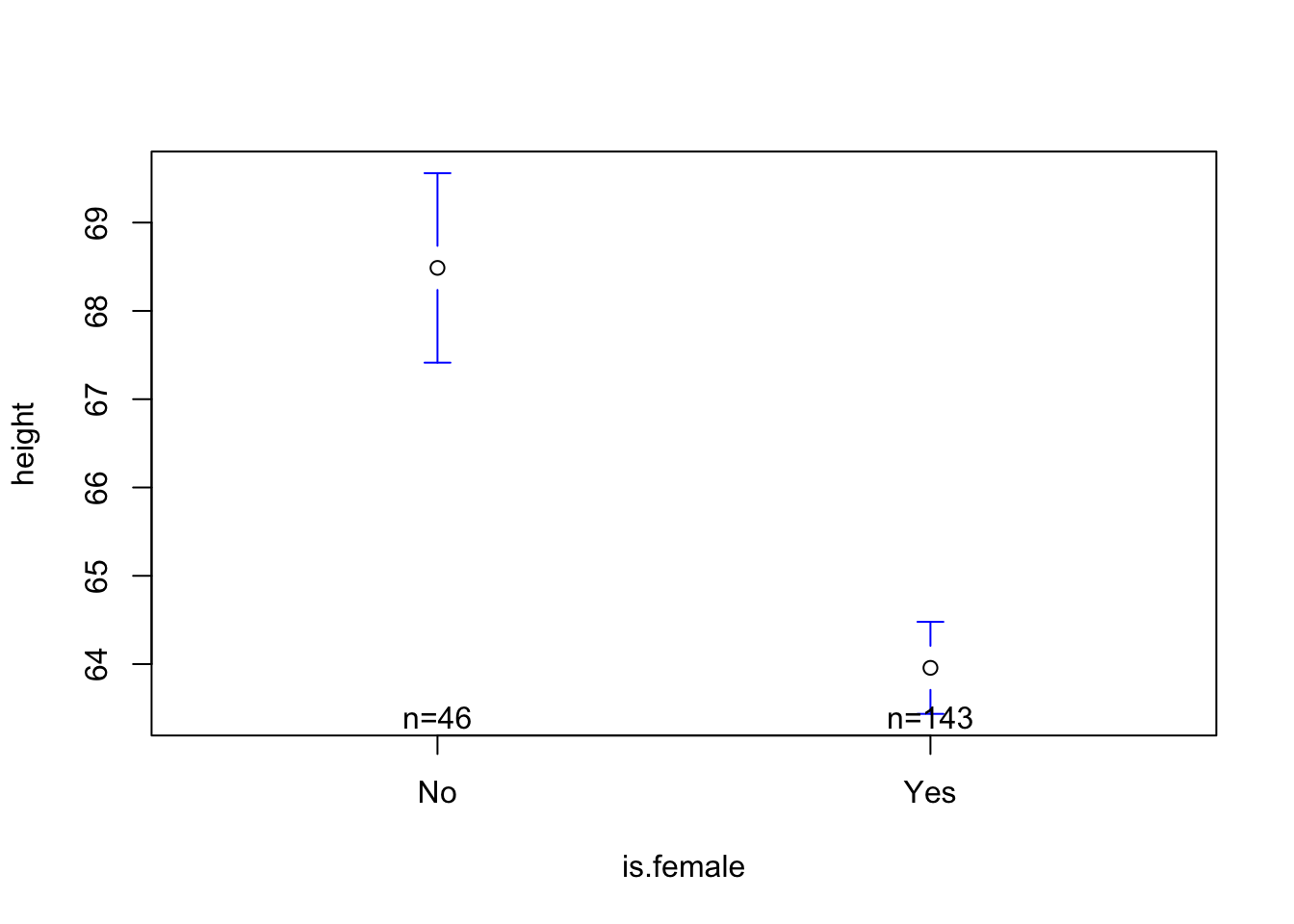
modb <- lm(height ~ is.female, data = d)
summary(modb)

Call:
lm(formula = height ~ is.female, data = d)

Residuals:
    Min      1Q  Median      3Q     Max 
-10.958  -1.958  -0.487   2.042   9.042 

Coefficients:
             Estimate Std. Error t value Pr(>|t|)    
(Intercept)   68.4870     0.4821 142.074  < 2e-16 ***
is.femaleYes  -4.5293     0.5542  -8.173 4.44e-14 ***
---
Signif. codes:  0 '***' 0.001 '**' 0.01 '*' 0.05 '.' 0.1 ' ' 1

Residual standard error: 3.269 on 187 degrees of freedom
  (10 observations deleted due to missingness)
Multiple R-squared:  0.2632,    Adjusted R-squared:  0.2592 
F-statistic: 66.79 on 1 and 187 DF,  p-value: 4.438e-14

plotmeans(height ~ is.female, data = d, connect = F)

height ~ long.hair + is.female

modc <- lm(height ~ long.hair + is.female, data = d)
## NO GRAPH FOR THE MULTIPLE REGRESSION
summary(modc)

Call:
lm(formula = height ~ long.hair + is.female, data = d)

Residuals:
    Min      1Q  Median      3Q     Max 
-10.097  -2.106  -0.180   1.894   8.894 

Coefficients:
             Estimate Std. Error t value Pr(>|t|)    
(Intercept)   68.1800     0.5156 132.239  < 2e-16 ***
long.hairYes   1.0086     0.6190   1.630    0.105    
is.femaleYes  -5.0828     0.6479  -7.845  3.3e-13 ***
---
Signif. codes:  0 '***' 0.001 '**' 0.01 '*' 0.05 '.' 0.1 ' ' 1

Residual standard error: 3.255 on 186 degrees of freedom
  (10 observations deleted due to missingness)
Multiple R-squared:  0.2736,    Adjusted R-squared:  0.2657 
F-statistic: 35.02 on 2 and 186 DF,  p-value: 1.235e-13

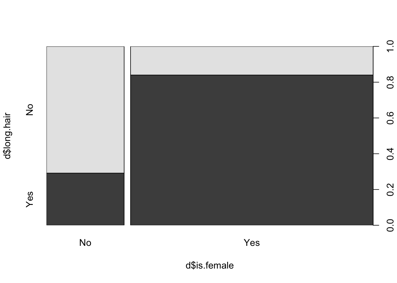
IV1 and IV2 are related to each other, and each related to the DV)

plot(d$long.hair ~ d$is.female)

Multiple Regression : Visualized in Multi-Dimensional Space!

The code below may not work on your computer; see lecture recording for an interpretation / explanation!

#install.packages('rgl')
#install.packages('car')
library(car)
library(rgl)

scatter3d(as.numeric(d$is.female), # IV1 - must be numeric (if not already)
          d$height, # DV
          as.numeric(d$long.hair)) # IV2 - must be numeric (if not already)

Reporting Effects in a Regression Table.

Table 1. Unstandardized Regression Coefficients; Predicting Height from Long.Hair and Is.Female.

	Model 1	Model 2	Model 3
Intercept
Long.Hair (0 = No; 1 = Yes)
Is.Female (0 = No; 1 = Yes)
\(R^2\)

There’s a Package in R For This!

# install.packages("jtools") # a new package!!!
library(jtools) # make sure you installed the new package first.
export_summs(moda, modb, modc,
             coefs = c("Long Hair (0 = No, 1 = Yes)" = "long.hairYes",
                       "Is Female (0 = No, 1 = Yes)" = "is.femaleYes"))

	Model 1	Model 2	Model 3
Long Hair (0 = No, 1 = Yes)	-1.59 **		1.01
	(0.61)		(0.62)
Is Female (0 = No, 1 = Yes)		-4.53 ***	-5.08 ***
		(0.55)	(0.65)
N	190	189	189
R2	0.03	0.26	0.27
*** p < 0.001; ** p < 0.01; * p < 0.05.

BREAK TIME : MEET BACK AT 4:40

Milestone #4 : Anyone want to share their project?