score Q1 Q2 Q3 Q4 Q5 Q6 Q7 Q8 Q9 Q10 Q11 Q12 Q13 Q14 Q15 Q16 Q17 Q18 Q19 Q20
1 18 2 2 2 2 1 2 1 2 2 2 1 1 2 1 1 1 2 1 1 1
2 6 2 2 2 1 2 2 1 2 1 1 2 2 2 1 2 2 1 1 2 1
3 27 1 2 2 1 2 1 2 1 2 2 2 1 1 1 1 1 2 2 1 1
4 29 1 1 2 2 2 1 2 1 1 2 1 1 1 1 1 1 2 2 1 2
5 6 1 2 1 1 1 2 1 2 1 2 2 2 2 2 1 1 1 1 1 1
6 19 1 2 2 1 2 1 1 1 2 2 1 1 1 2 1 1 1 1 1 1
Q21 Q22 Q23 Q24 Q25 Q26 Q27 Q28 Q29 Q30 Q31 Q32 Q33 Q34 Q35 Q36 Q37 Q38 Q39
1 1 1 1 2 2 2 1 2 2 2 1 2 1 1 1 2 2 2 1
2 2 2 1 2 2 2 2 1 2 2 2 1 2 2 1 2 2 2 2
3 2 2 2 2 1 2 1 1 2 1 2 2 1 1 2 1 1 2 1
4 1 1 1 2 1 2 1 2 2 1 1 2 1 1 2 1 2 2 1
5 1 2 1 2 2 1 2 1 2 2 2 1 2 2 1 2 2 2 0
6 1 1 1 1 2 1 1 1 2 1 1 2 1 2 1 1 2 2 2
Q40 elapse gender age
1 2 211 1 50
2 1 149 1 40
3 2 168 1 28
4 1 230 1 37
5 1 389 1 50
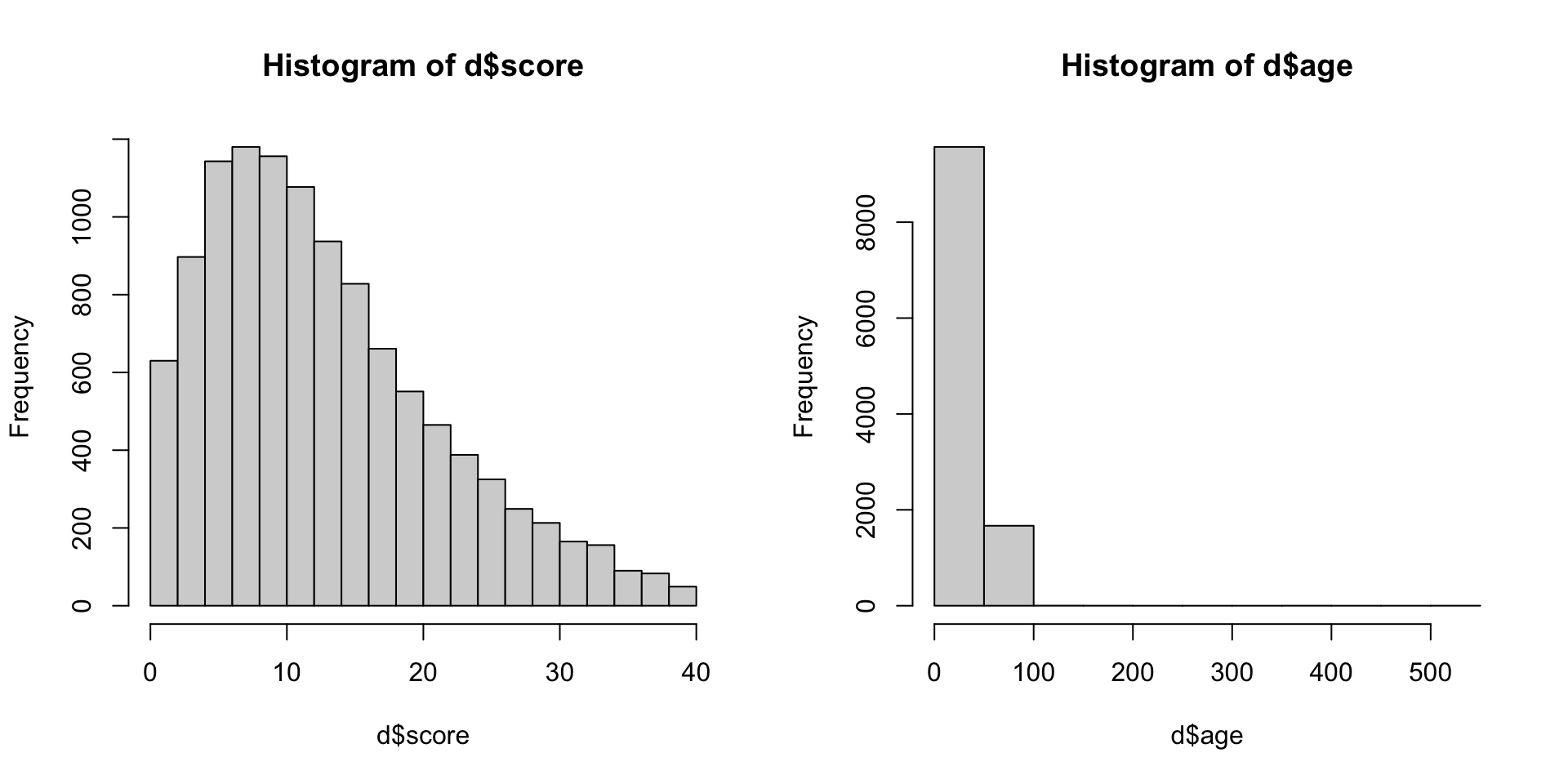
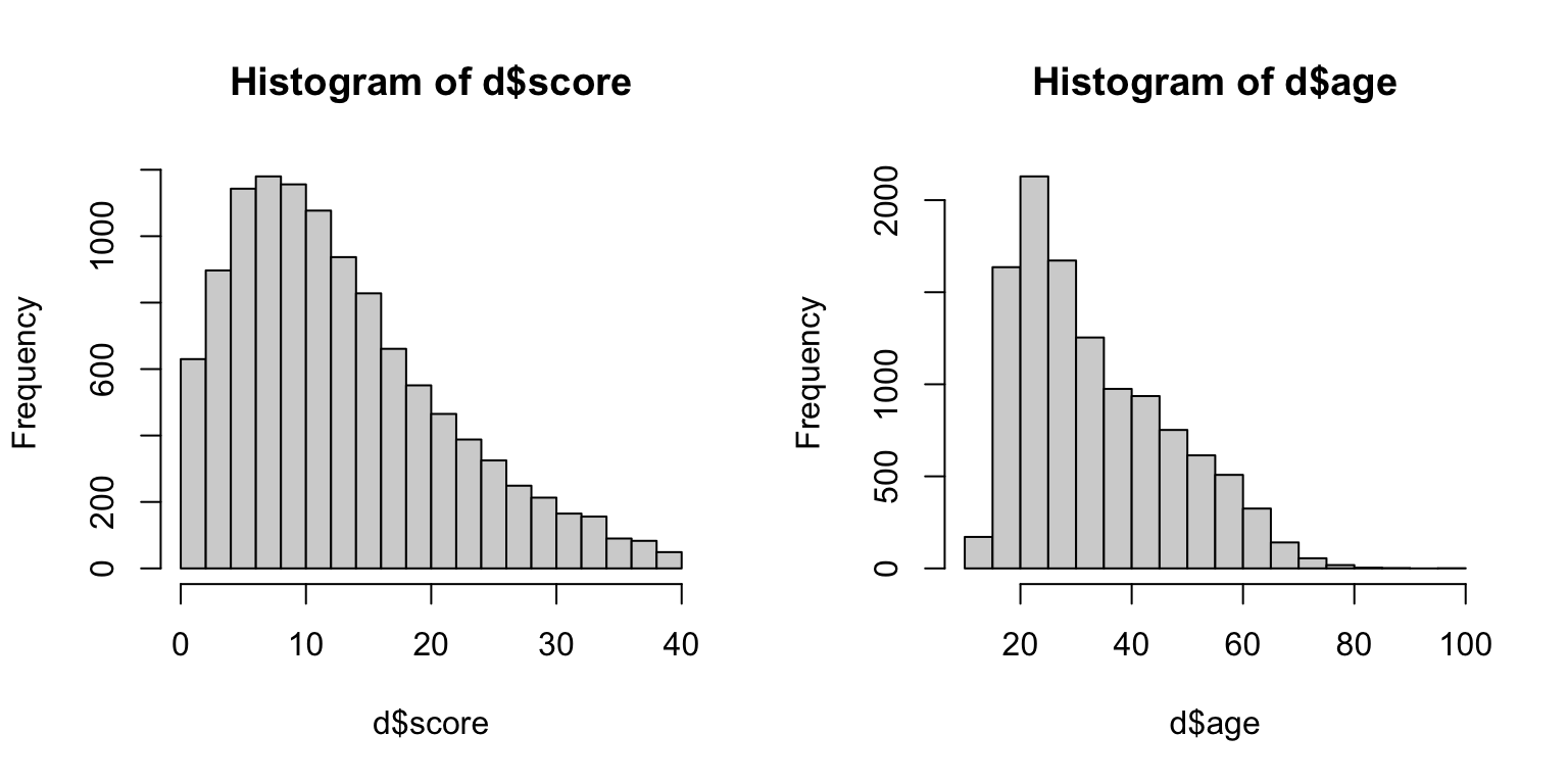
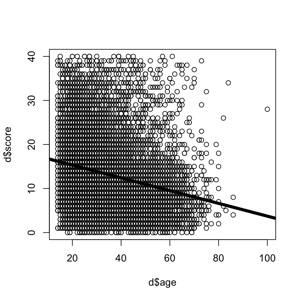
6 2 361 1 27CHECK-IN : Is there a relationship between narcissism and age?
- score = narcissism score (40-item scale)
- age = Entered as a free response. Ages below 14 have been ommited from the dataset.
- sex = Chosen from a drop down list (1=male, 2=female, 3=other; 0=none was chosen).

Check-In Spoilers
- score = narcissism score (40-item scale)
- age = Entered as a free response. Ages below 14 have been ommited from the dataset.
- sex = Chosen from a drop down list (1=male, 2=female, 3=other; 0=none was chosen).

BREAK TIME : A Quick Study
- No talking, no looking up answers!
- Will use data in lecture :)

RECAP : \(R^2\) In Real-Life

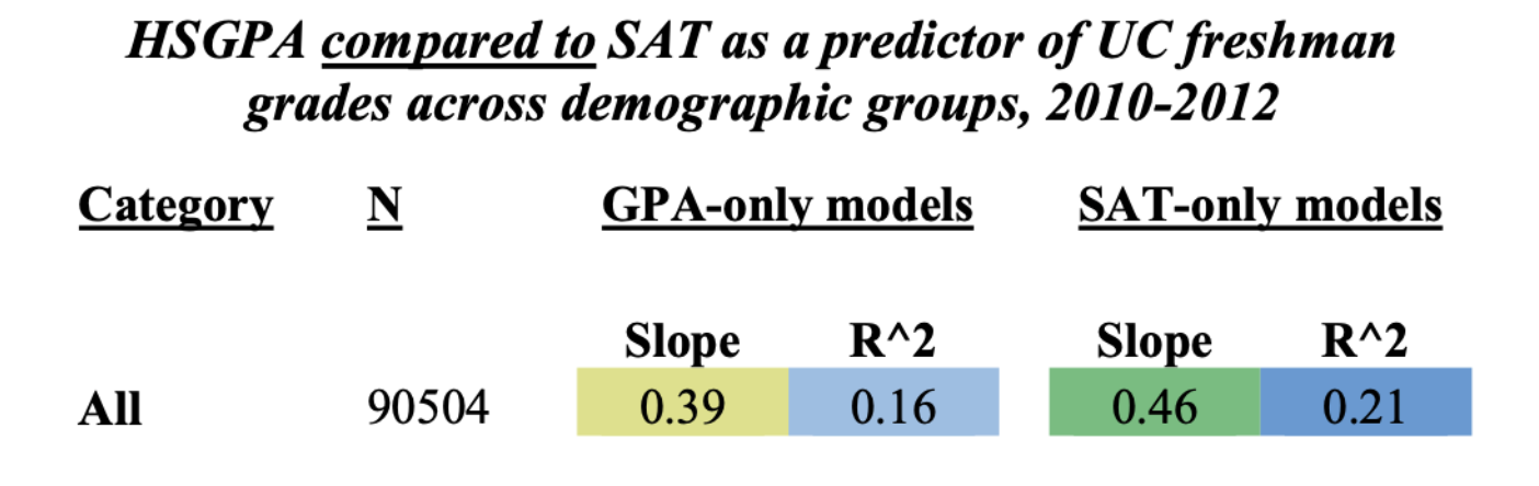
DISCUSS : what do these linear models tell us about the relationship between GPA, SAT (IVs) and freshman grades (DV)?
Your Survey : Likert Scales
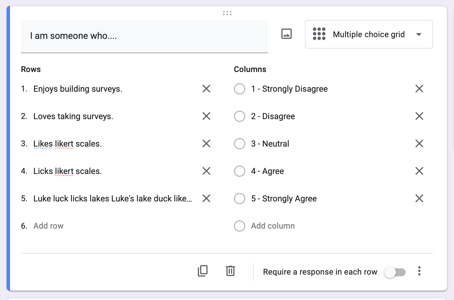
Use a Multiple Choice Grid
- Each row is an item.
- All the items use the same “stem” (“I am someone who…”)
- Do not require responses. Okay if folks skip, right?
- Attention Checks (e.g., “Mark Strongly Agree for this question.”)
- BETTER : to keep the survey short; give authentic motivation.
- Each column is a response. Use a 1-5 scale to make it easy / allow for neutral.
Your Survey : Categorical Variables

- Include demographic variables like age and sex; give people options to self-identify as something outside a forced binary!
- Keep categorical variables to just a few levels; you will need a LOT of data to capture variation if there are too many levels! 3-4 groups per variable.
Your Survey : The Right Type of Variable!
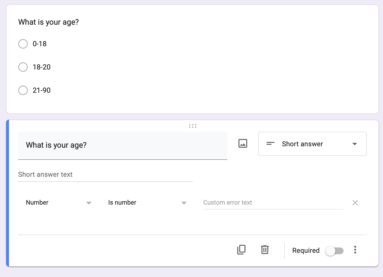
Make sure categorical variables are not better measured numerically. set “response validation” for any open-ended numbers you hope to collect to make data cleaning easier.
Make sure each variable is measured independently of the others. For example, if I want to measure the relationship between happiness and reading, I would want to measure these separately.
- I am happy.
- I like to read.
Reading makes me happy.This mixes up the two variables (the DV and IV). It could be a cool measure on its own (love for reading scale?).
THE END.
