Introduction to Linear Models
CHECK-IN : Post Mini-Exam Survey!

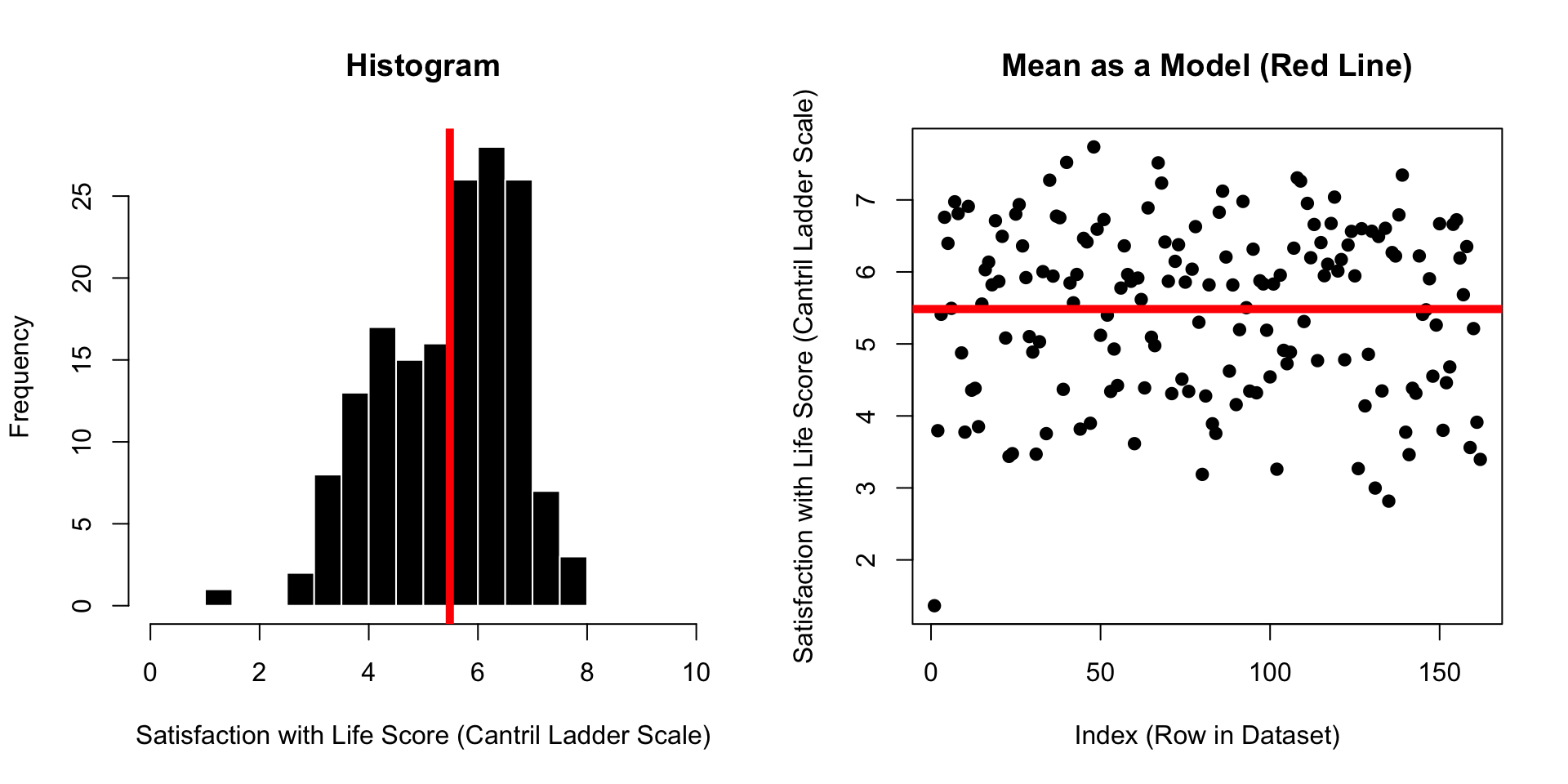
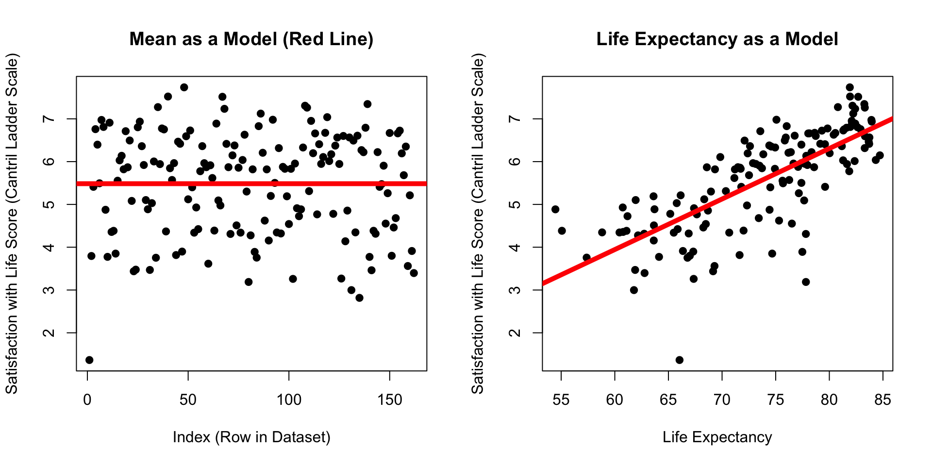
RECAP : The Mean as Prediction?
\(\huge y_i = \hat{Y} + \epsilon_i\)
\(\Large y_i\) = the DV = the individual’s actual score we are trying to predict.
on the graph: each individual dot
\(\Large \hat{Y}\) = our prediction (the mean).
on the graph: the solid red line
\(\Large \epsilon\) = residual error = difference between predicted and actual values of y
on the graph: the distance between each dot and the line.

RECAP : The Mean as Prediction With Error
\(\huge \epsilon_i = y_i - \hat{Y}\)
Error = actual score - prediction (the mean)
[1] 233.827- This number is critical - quantified error in our prediction.
- This number makes no sense (total unsquared error??!?!)
- sd gives some context (average error)
- use number as a starting place to see if we can make better predictions
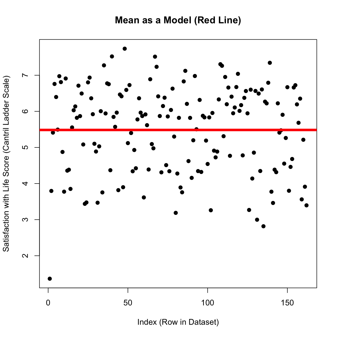
KEY IDEA : The mean is an okay starting place for our predictions, but we can try to do better!
| the mean | the linear model ™ © |
 |
 |
DISCUSS : Making Predictions
THINK ABOUT A LINEAR MODEL : how do you think the variables (below) would help (or not help) us predict the happiness of a country in 2024? Why / why not???
THINK ABOUT SOURCES OF DATA. What other variables do you think would be important to include in this dataset?

TIME TO PLAY : WHERE’S THE LINE
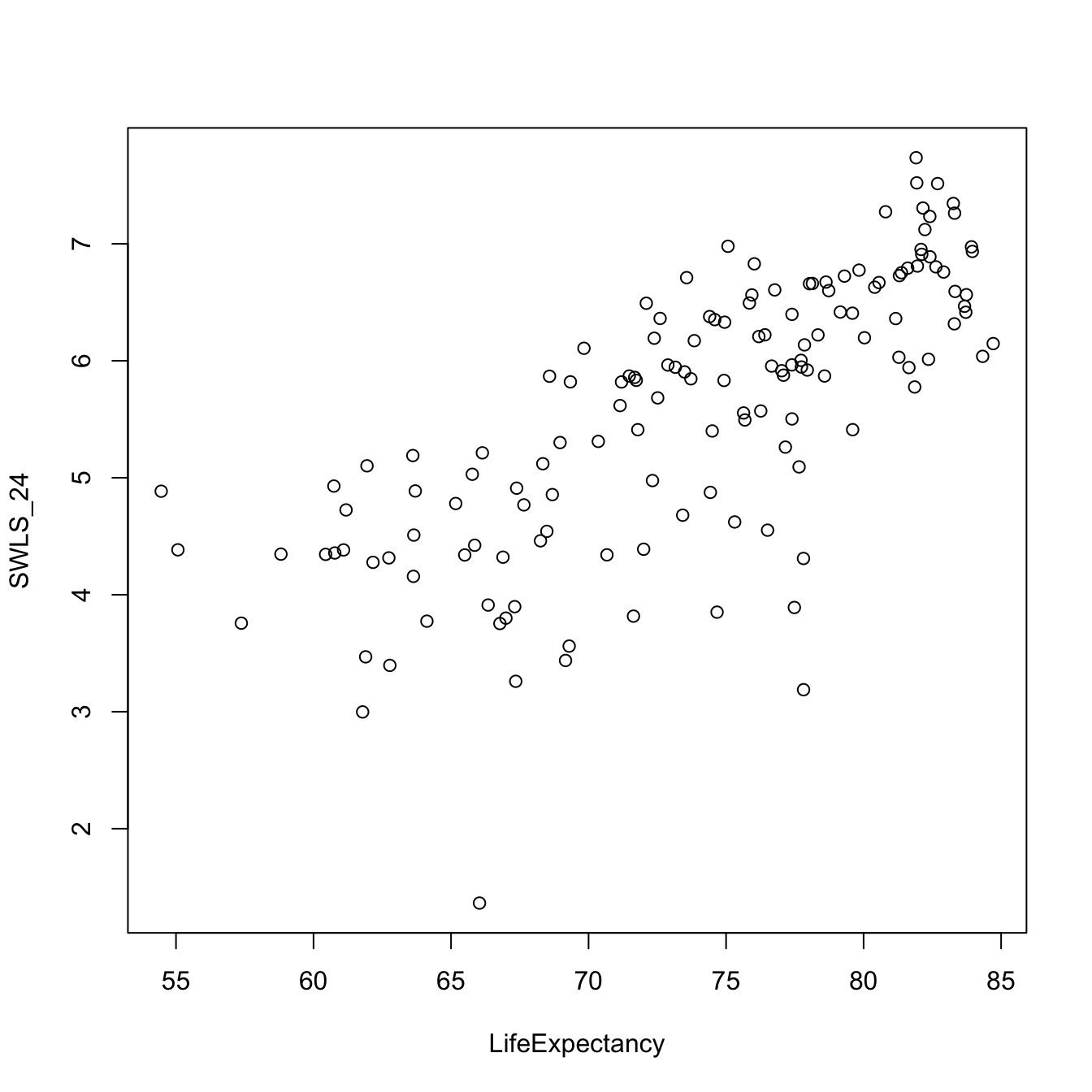
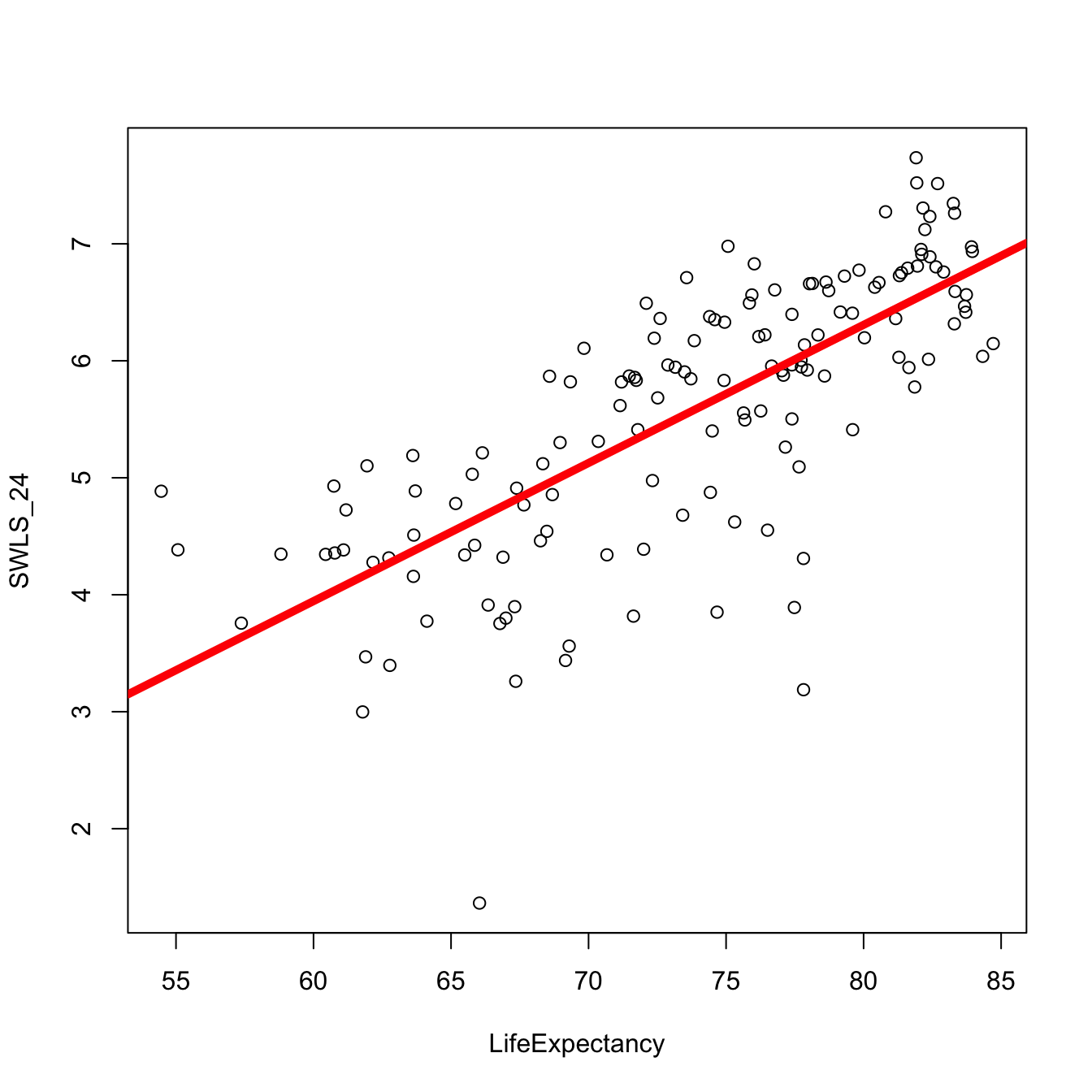
What’s Going On : It’s a Line
\(\Huge y_i = a + b_1 * X_i + \epsilon_i\)
   (Intercept) LifeExpectancy
-3.14 0.12 
\(\Large y_i\) = the DV = each actual score on the DV.
on the graph:** each dot on the y-axis
\(\Large a\) = the intercept = starting place for our prediction (“the predicted value of y when all x values are zero”.)
on the graph:** the value of the line at X = 0
\(\Large X_i\) = the IV = the actual score on the IV.
on the graph: the value of each dot on the x-axis
\(\Large b_1\) = the slope = an adjustment to our prediction of y based changes in x
on the graph: how much the line increases in y value when x-values increase by 1 unit.
\(\Large \epsilon_i\) = residual error = the distance between actual y and predicted y
on the graph: the distance between each individual data point and the line.
The Linear Model : Error in Our Predictions
Which model has dots that are closer to the line??? (Mean of Satisfaction or Life Expectancy)

The Linear Model : Quantifying Error


BREAK TIME : MEET BACK AT 3:30

Milestone #2 (Measures)
The Likert Scale
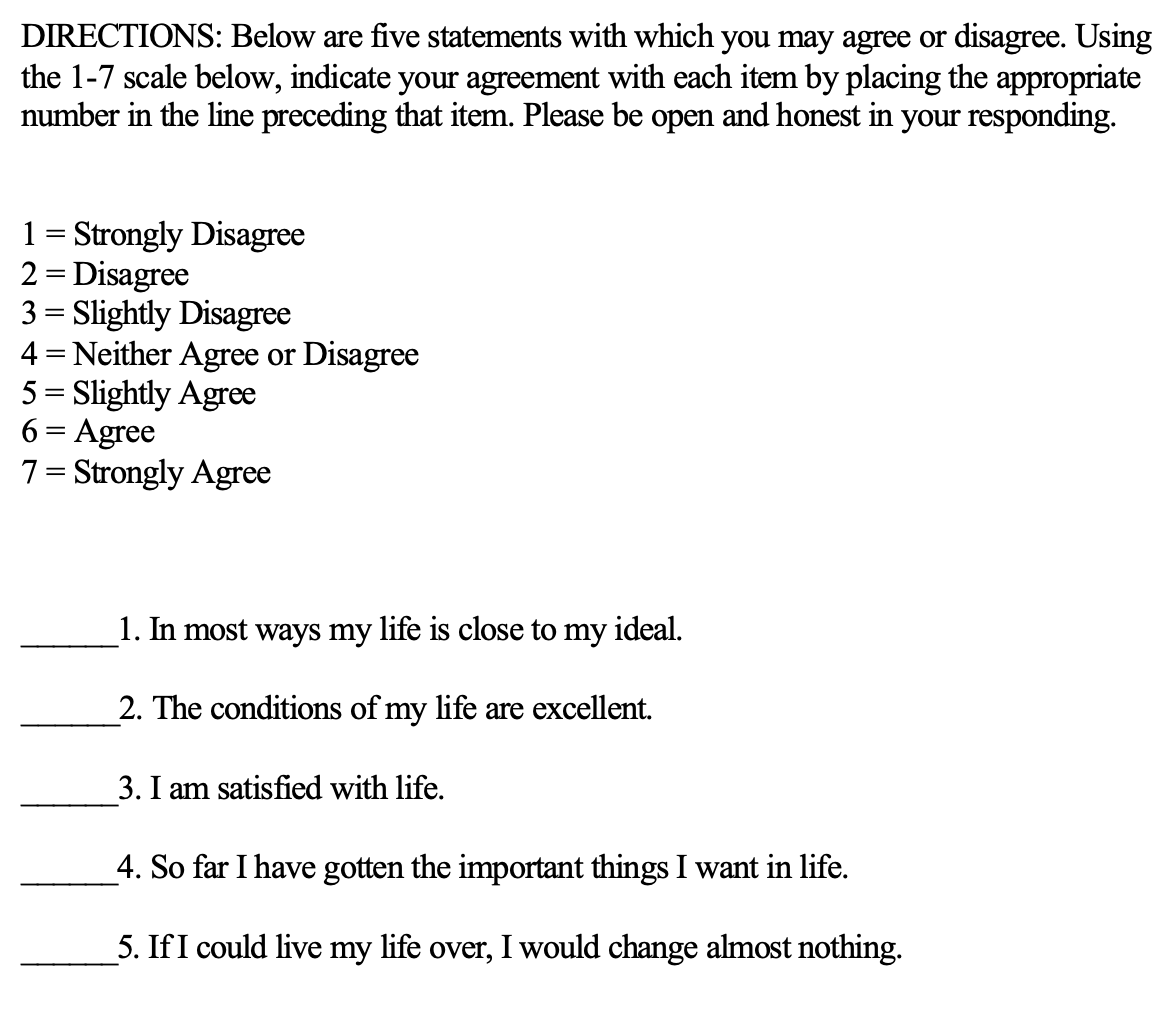
Example : Satisfaction With Life Scale
scale : The variable that you want to measure as a continuous variable.
items : The specific question(s) in the scale. Each item measures some aspect of the variable the researcher is interested in.
positively keyed items : An item that measures the high end of the scale, where answering “yes” to the question means you are high on this variable.
negatively keyed items : An item that measures the low end of the scale, where answering “yes” to the question means you are low on the variable.
response scale : How people answer the scale items.