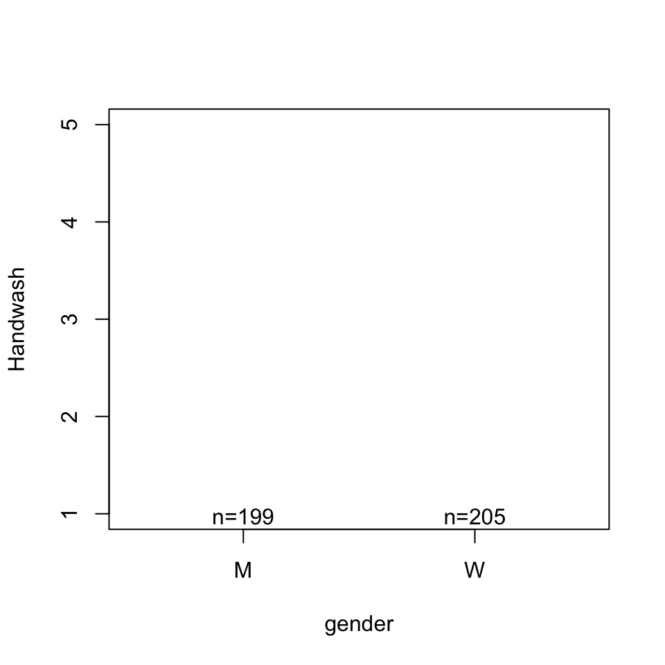
Call:
lm(formula = Handwash ~ gender, data = d)

Residuals:
    Min      1Q  Median      3Q     Max
-3.5659 -0.5659  0.4341  0.7437  0.7437

Coefficients:
            Estimate Std. Error t value Pr(>|t|)
(Intercept)  3.25628    0.06065  53.688  < 2e-16 ***
genderW      0.30957    0.08515   3.636 0.000313 ***
---
Signif. codes:  0 '***' 0.001 '**' 0.01 '*' 0.05 '.' 0.1 ' ' 1

Residual standard error: 0.8556 on 402 degrees of freedom
  (438 observations deleted due to missingness)
Multiple R-squared:  0.03184,   Adjusted R-squared:  0.02943
F-statistic: 13.22 on 1 and 402 DF, p-value: 0.0003131Welcome Back :)
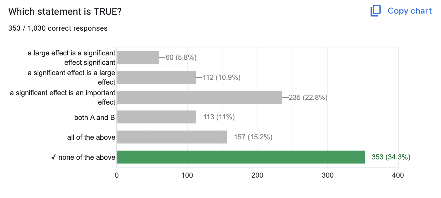
Check-In (No R Needed): Testing Theories
The Vibe

NHST Review.
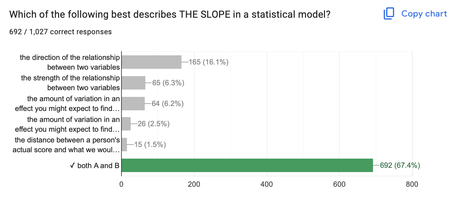
- Slope
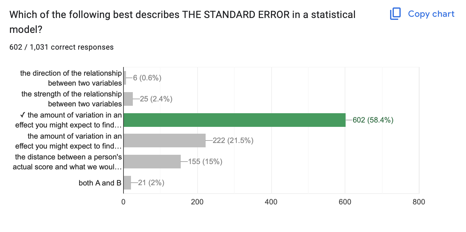
- Standard Error
- Significance is Not…
- Significance is Not
- Significance Is…
- …Confusing.
- Other Questions?
- Direction & Strength of a Relationship
- Hard to evaluate strength across models if the units differ too.
- The amount of variation in an effect you might expect to find due to chance if the null hypothesis were “true”.
- …about slope! Large slope & sampling error = NOT SIGNIFICANT
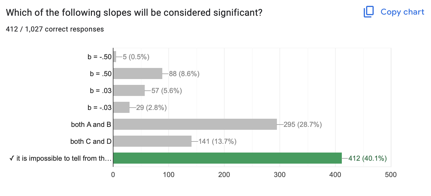
- …about size : you can be VERY confident that a small effect is not due to sampling error.
- …about importance : why does the effect matter?
- …about truth : our estimates of sampling error are all made up.
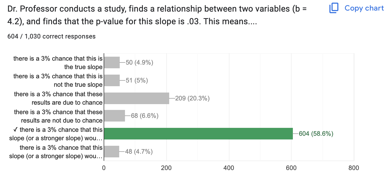
A p-value of .03 means…there is a 3% chance that this slope (or a stronger slope) would be found due to chance if the true correlation was zero.
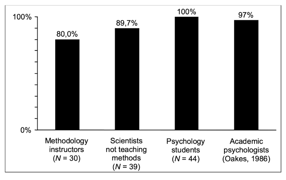
Haller, H., & Krauss, S. (2002). Misinterpretations of significance: A problem students share with their teachers. Methods of Psychological Research, 7(1), 1-20.
More Practice
Evaluate the relationships between the variables (slope, significance, importance)
Is there a relationship between narcissism (DV = NPI) and testosterone?
Call:
lm(formula = NPI ~ test, data = h)

Residuals:
     Min       1Q   Median       3Q      Max
-1.29549 -0.36339 -0.02748  0.27697  1.36124

Coefficients:
            Estimate Std. Error t value Pr(>|t|)
(Intercept) 2.882071   0.126950  22.702   <2e-16 ***
test        0.003894   0.001502   2.593   0.0112 *
---
Signif. codes:  0 '***' 0.001 '**' 0.01 '*' 0.05 '.' 0.1 ' ' 1

Residual standard error: 0.5375 on 84 degrees of freedom
  (36 observations deleted due to missingness)
Multiple R-squared:  0.07414,   Adjusted R-squared:  0.06311
F-statistic: 6.726 on 1 and 84 DF,  p-value: 0.01121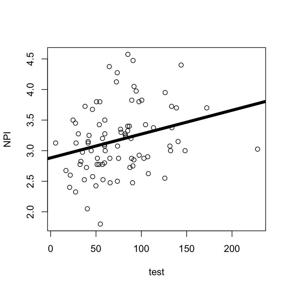
Is there a relationship between narcissism (DV = NPI) and sex?
Call:
lm(formula = NPI ~ sex, data = h)

Residuals:
     Min       1Q   Median       3Q      Max
-1.47375 -0.34557 -0.02989  0.36079  1.36397

Coefficients:
            Estimate Std. Error t value Pr(>|t|)
(Intercept)   3.5365     0.1478  23.925   <2e-16 ***
sex          -0.2627     0.1074  -2.446    0.016 *
---
Signif. codes:  0 '***' 0.001 '**' 0.01 '*' 0.05 '.' 0.1 ' ' 1

Residual standard error: 0.5245 on 112 degrees of freedom
  (8 observations deleted due to missingness)
Multiple R-squared:  0.05073,   Adjusted R-squared:  0.04225
F-statistic: 5.985 on 1 and 112 DF,  p-value: 0.01598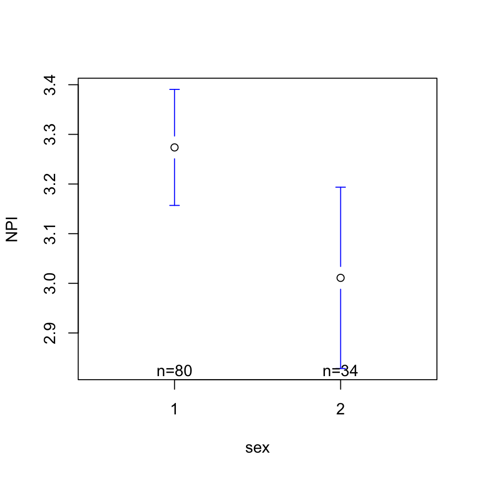
Is there a relationship between testosterone (DV = test) and sex?
Call:
lm(formula = test ~ sex, data = h)

Residuals:
    Min      1Q  Median      3Q     Max
-60.144 -17.211  -3.365  12.111 137.486

Coefficients:
            Estimate Std. Error t value Pr(>|t|)
(Intercept)  139.972      9.935  14.088  < 2e-16 ***
sex          -49.288      7.208  -6.838 1.01e-09 ***
---
Signif. codes:  0 '***' 0.001 '**' 0.01 '*' 0.05 '.' 0.1 ' ' 1

Residual standard error: 31.34 on 88 degrees of freedom
  (32 observations deleted due to missingness)
Multiple R-squared:  0.347, Adjusted R-squared:  0.3396
F-statistic: 46.76 on 1 and 88 DF,  p-value: 1.014e-09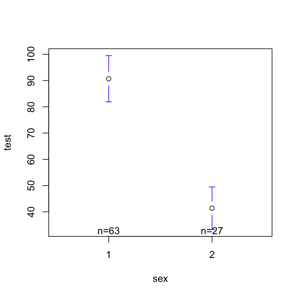
In models 1-3, we wee
- Testosterone is related to narcissism.
- Sex is related to testosterone.
- Sex and testosterone are related to each other……
In models 1-3, we wee
- Testosterone is related to narcissism.
- Sex is related to testosterone.
- Sex and testosterone are related to each other……
Call:
lm(formula = NPI ~ sex + test, data = h)

Residuals:
     Min       1Q   Median       3Q      Max
-1.31150 -0.36048 -0.02691  0.27507  1.35277

Coefficients:
             Estimate Std. Error t value Pr(>|t|)
(Intercept)  2.946551   0.315506   9.339 1.37e-14 ***
sex         -0.034852   0.155946  -0.223   0.8237
test         0.003646   0.001875   1.944   0.0552 .
---
Signif. codes:  0 '***' 0.001 '**' 0.01 '*' 0.05 '.' 0.1 ' ' 1

Residual standard error: 0.5405 on 83 degrees of freedom
  (36 observations deleted due to missingness)
Multiple R-squared:  0.07469,   Adjusted R-squared:  0.0524
F-statistic:  3.35 on 2 and 83 DF,  p-value: 0.03989
BREAK TIME : MEET BACK AT 3:45

RECAP : Likert Scale (Self-Esteem)
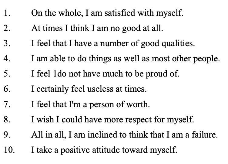
items : The specific question(s) in the scale. Each item measures some aspect of the variable the researcher is interested in.
positively keyed items : An item that measures the high end of the scale, where answering “yes” to the question means you are high on this variable.
negatively keyed items : An item that measures the low end of the scale, where answering “yes” to the question means you are low on the variable.
response scale : How people answer the scale items.
IN R : Three Steps
  Q1 Q2 Q3 Q4 Q5 Q6 Q7 Q8 Q9 Q10 gender age source country
1  3  3  1  4  3  4  3  2  3   3      1  40      1      US
2  4  4  1  3  1  3  3  2  3   2      1  36      1      US
3  2  3  2  3  3  3  2  3  3   3      2  22      1      US
4  4  3  2  3  2  3  2  3  3   3      1  31      1      US
5  4  4  1  4  1  4  4  1  1   1      1  30      1      EU
6 4 4 1 3 1 3 4 2 2 1 2 25 1 CA 1 2 3 4 NA's
3011 8647 21018 15200 98 [1] 47974 Q1 Q2 Q4 Q6 Q7 Q3 Q5 Q8 Q9 Q10
1 3 3 4 4 3 4 2 3 2 2
2 4 4 3 3 3 4 4 3 2 3
3 2 3 3 3 2 3 2 2 2 2
4 4 3 3 3 2 3 3 2 2 2
5 4 4 4 4 4 4 4 4 4 4
6 4 4 3 3 4 4 4 3 3 4
Reliability analysis
Call: psych::alpha(x = SELFES.DF)

  raw_alpha std.alpha G6(smc) average_r S/N     ase mean  sd median_r
      0.91      0.91    0.92      0.52  11 0.00058  2.6 0.7     0.52

    95% confidence boundaries
         lower alpha upper
Feldt     0.91  0.91  0.91
Duhachek  0.91  0.91  0.91

 Reliability if an item is dropped:
    raw_alpha std.alpha G6(smc) average_r  S/N alpha se  var.r med.r
Q1       0.90      0.90    0.91      0.51  9.5  0.00064 0.0089  0.51
Q2       0.91      0.91    0.91      0.52  9.7  0.00063 0.0085  0.52
Q4       0.91      0.91    0.91      0.53 10.3  0.00061 0.0081  0.53
Q6       0.90      0.90    0.90      0.50  9.2  0.00067 0.0087  0.51
Q7       0.90      0.90    0.91      0.51  9.3  0.00066 0.0089  0.51
Q3       0.90      0.90    0.91      0.51  9.3  0.00066 0.0094  0.51
Q5       0.90      0.91    0.91      0.52  9.6  0.00065 0.0098  0.51
Q8       0.91      0.91    0.92      0.54 10.7  0.00059 0.0064  0.54
Q9       0.90      0.91    0.91      0.52  9.6  0.00065 0.0085  0.52
Q10      0.90      0.90    0.90      0.51  9.3  0.00067 0.0086  0.51

 Item statistics
        n raw.r std.r r.cor r.drop mean   sd
Q1  47876  0.76  0.77  0.75   0.70  3.0 0.87
Q2  47658  0.73  0.74  0.71   0.66  3.1 0.79
Q4  47751  0.66  0.68  0.62   0.59  2.9 0.81
Q6  47809  0.81  0.81  0.79   0.75  2.6 0.92
Q7  47758  0.79  0.79  0.77   0.74  2.4 0.93
Q3  47751  0.79  0.79  0.76   0.73  2.7 0.95
Q5  47781  0.76  0.76  0.72   0.69  2.6 0.98
Q8  47797  0.64  0.63  0.56   0.54  2.3 0.96
Q9  47728  0.76  0.75  0.73   0.69  2.2 0.99
Q10 47772  0.81  0.80  0.78   0.74  2.4 1.07

Non missing response frequency for each item
       1    2    3    4 miss
Q1  0.06 0.18 0.44 0.32 0.00
Q2  0.04 0.13 0.50 0.33 0.01
Q4  0.05 0.21 0.50 0.24 0.00
Q6  0.14 0.33 0.37 0.17 0.00
Q7  0.18 0.34 0.35 0.14 0.00
Q3  0.13 0.28 0.37 0.22 0.00
Q5  0.14 0.32 0.32 0.22 0.00
Q8  0.21 0.41 0.24 0.14 0.00
Q9  0.27 0.40 0.20 0.14 0.01
Q10 0.24 0.33 0.22 0.22 0.00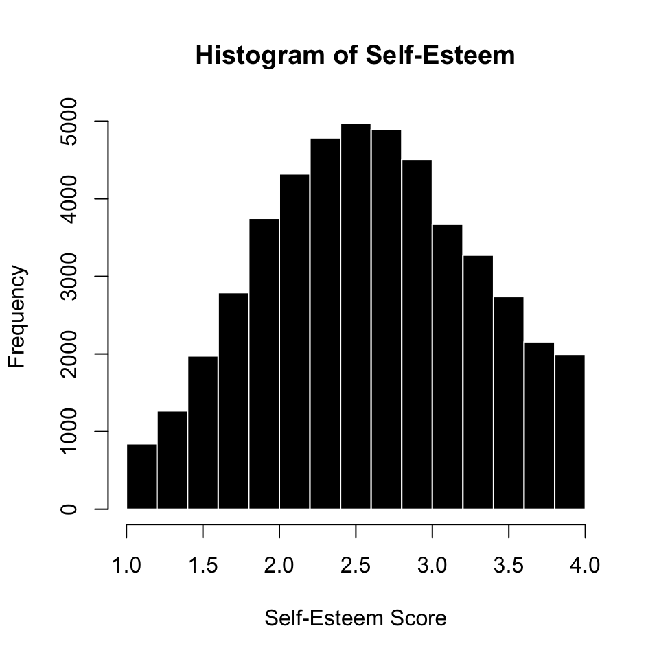
THE END.