4:45 - ????. The Learning is Over; Would You Like to Learn More???
Announcements
No Final Exam. Yay.
Final Project Due 12/13 at 11:59 PM. Late submissions risk an incomplete in the class. Incomplete grades\s are only given for students missing the final project, but otherwise passing the class. I am sorry that it is so hard to be a Berkeley student sometimes <3
“Done is better than perfect”. Prioritize the most important things; set reasonable expectations for yourself and boundaries for the time that you have (e.g., lit review can be superficial; okay if you can’t figure out how to create a scale, just
Make it clear how and where you are doing the work. Label your sections with headers; make sure your tables and graphs are visible.
There is no “right” way to do the study. We want to see evidence that you tried and are learning. (But see the rubric.)
Keep it simple.
Simple measures :
okay to use one measure of your DV even thought you had two.
okay to simplify your categorical variable (e.g., “which of these 15 music types do you love the most” –> “do you like experimental jazz (0 = no; 1 = yes)”)
Simple models : okay to just
Discussion Section : summary of ways that you could have (or should have) been more complicated in the Discussion Section
Appendix : List of all your measures. Good practice to be fully transparent about what you measured in the study.
Use paragraphs and headers to guide the reader.
Each new idea is a new paragraph. No solid wall of text please!
Headers help orient your reader to the different contents.
More Writing
The Abstract : the TLDR of your paper
Components of an Abstract :
1-2 sentences : what is your topic and why should we care?
1-2 sentences : what did you measure / do in your study?
1-2 sentences : what did you find?
1-2 sentences : why does this matter?
Activity : Write an Abstract for Each Other
Professor and Student Example Goes Here :
YOUR TURN!
The Discussion Section : Two Paragraphs Minimum!
Summary of Results (and Future Studies) :
What you found (NO STATS)
Why this matters / how this knowledge could be used / what other questions you might ask in the future?
Limitations and Future Directions
What would you do differently in your study?
How could (or should) future research address these limitations, and why would that be important to do?
The Rich Lyons is our chancellor and the professor of this class has Invited me to give a Distinguished GoBears Guest Lecture
Student Example Goes Here
Student Example Goes Here
Student Example Goes Here
BREAK TIME : MEET BACK AT 4:45
The Learning is Over; Would You Like to Learn More?
Things to Remember in 50 Years
1. YouCanLearn Statistics and Computers : It is a process :)
check-in graph goes here.
2. Life is Complex : Psychology Tries to Use Statistics to Study Complexity
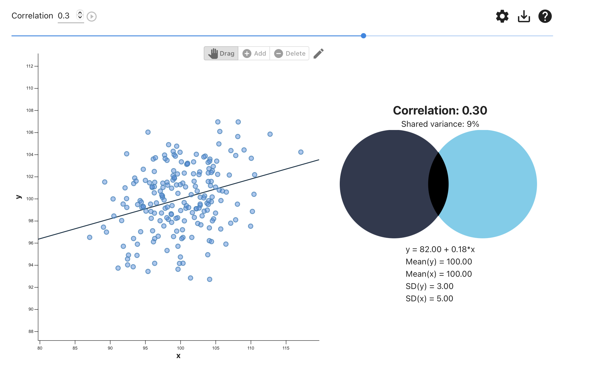
2A. Linear Models Make Predictions (with Errors)
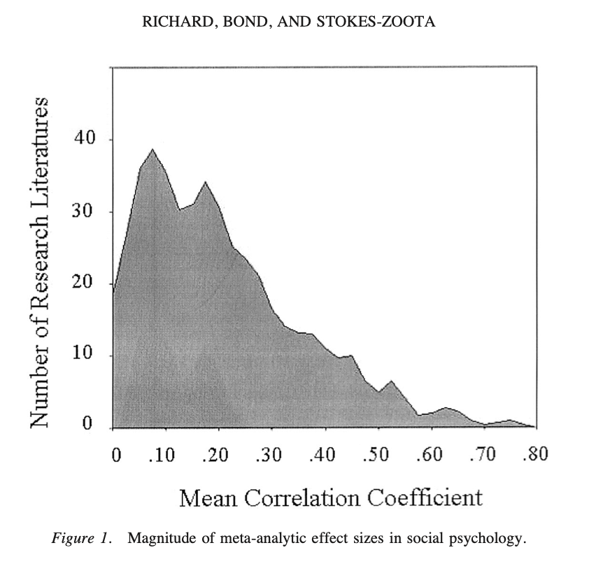
Hard to quantify; but best estimates that the average correlation between two variables is r < .30
Richard, F. D., Bond Jr, C. F., & Stokes-Zoota, J. J. (2003). One hundred years of social psychology quantitatively described. Review of general psychology, 7(4), 331-363.
But also, remember that a “correlation” / slope could look like any of the following graphs [Anscombe’s Quartet]
2B. Not Just Error in our Models…researchers are biased too.
Bias
Your Final Project Experiences?
previous beliefs bias. we are more likely to believe data that supports our results.
Did you study something that was personally relevant to you? (“Me-search”)
Clap : Yes / No
positive evidence. we seek out information in ways that supports our beliefs.
Was your theory (the “alternative”) something that you personally believe? Did you look for, or include, research in your introduction that did not support your theory?
clap : yes / no
availability bias. we are more likely to believe memorable or recent data.
How did you feel when your results were significant? When your results were not significant?
clap : happy / neutral / sad
social influence. we believe things others (w/ status) do.
Were you influenced by the topics or methods your friends / classmates were doing?
Did you trust research articles that were more recent and / or highly cited (higher citation counts)?
Clap : Yes / No
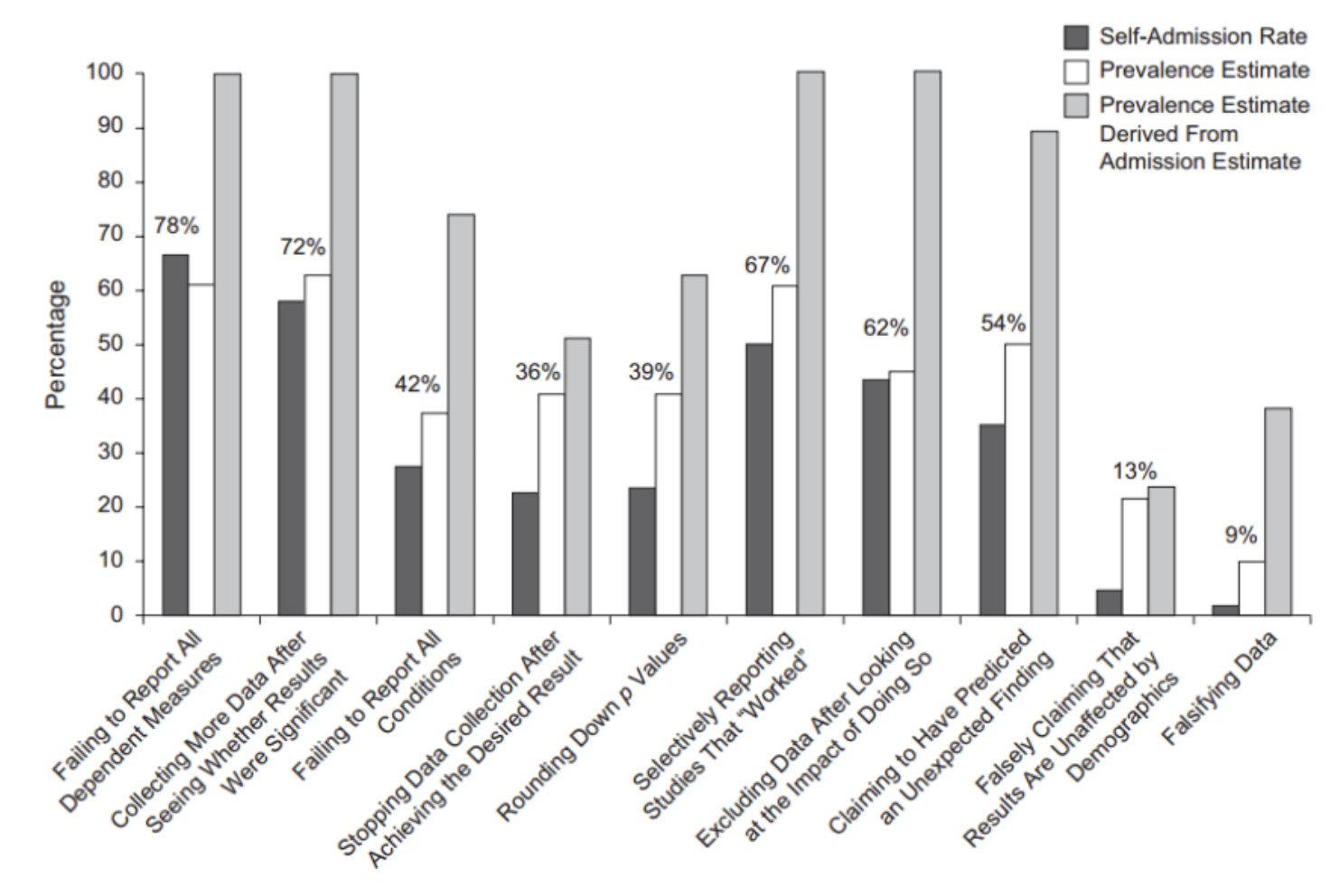
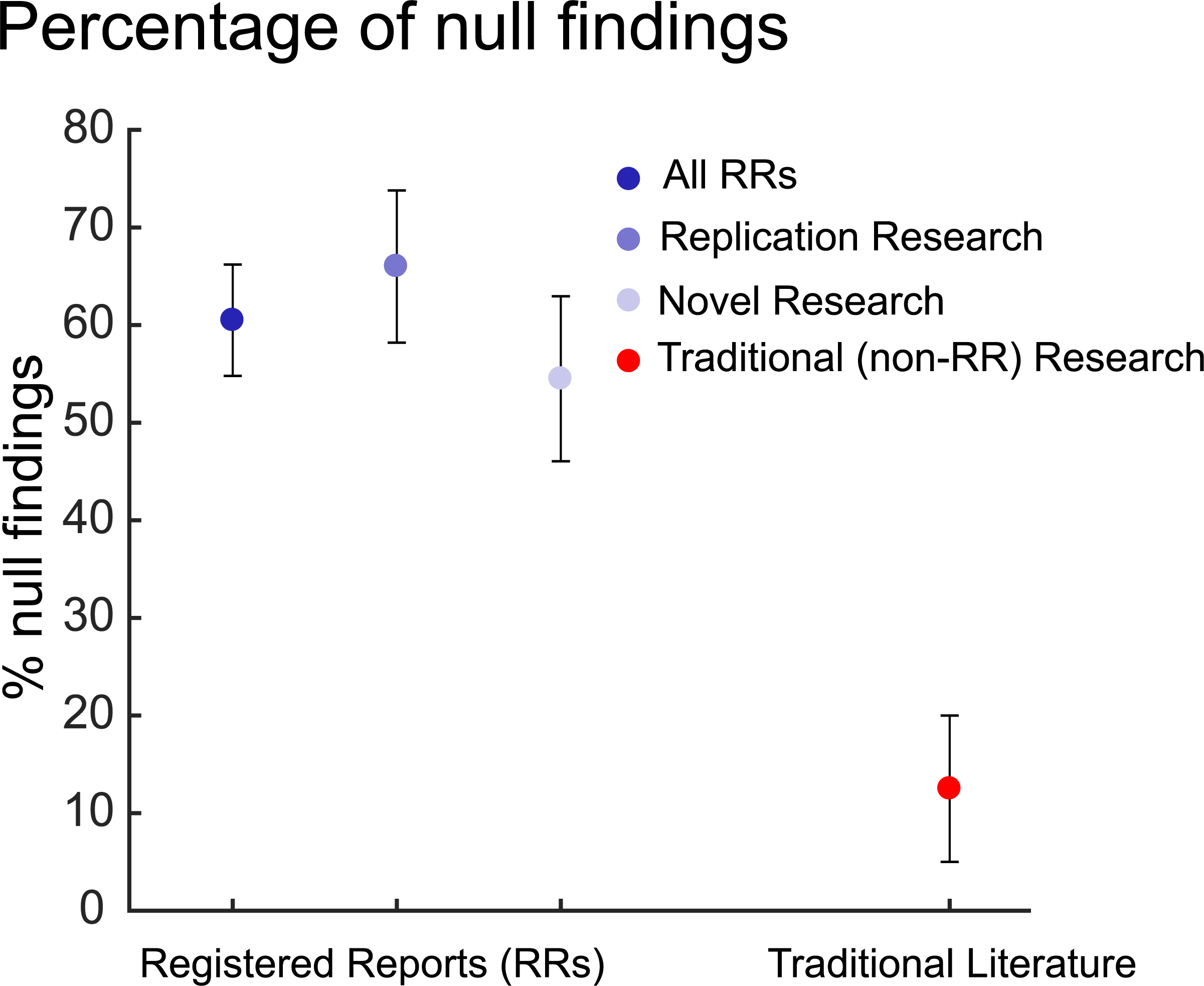
2C. Oh and our Methods and Measures Are Biased….Maybe All of Science is Biased?
p-hacking : making changes to your model or data in order to “get” your p-values.
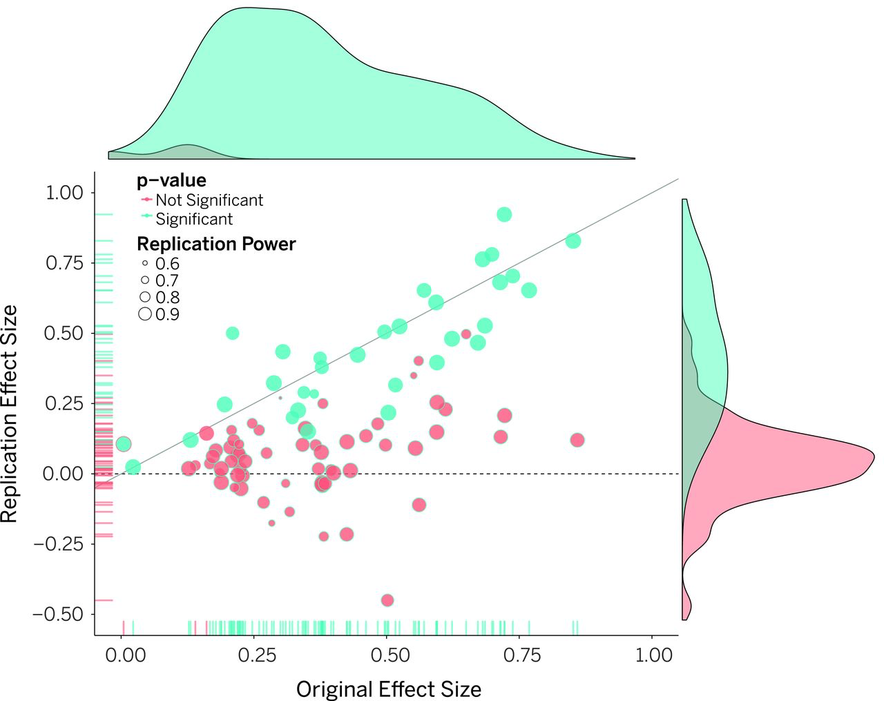
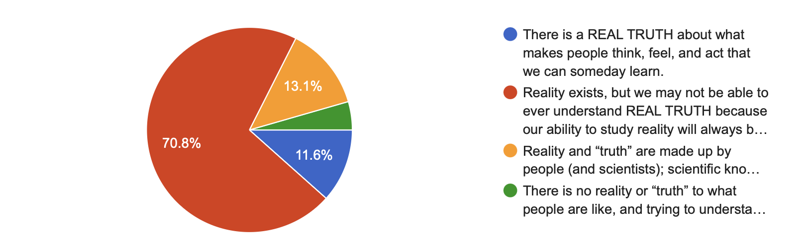
2E. But wait…is there even a “TRUTH” about what people are like?
Beginning of Semester
End of Semester
Things to Immediately Forget (or Learn More About)
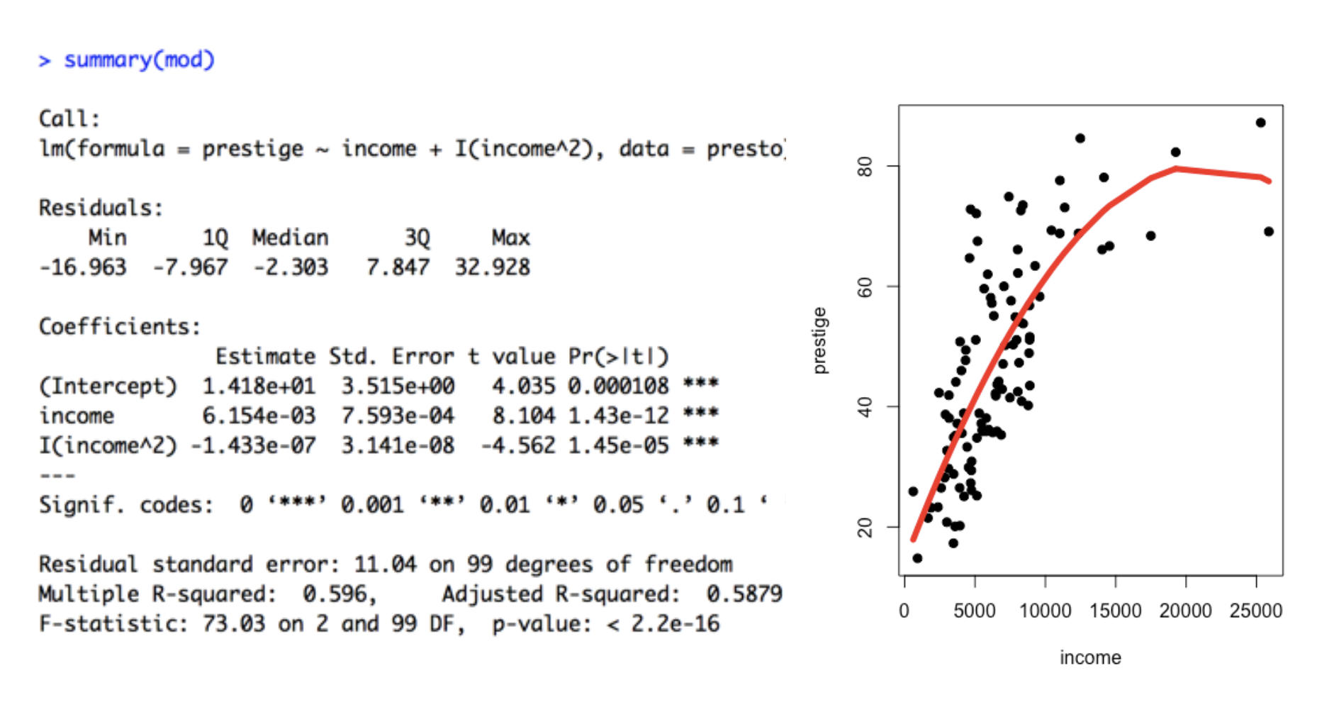
1. Quadratic Effects : A Regression Line Can Bend
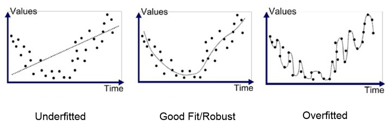
But careful about overfitting….
2. Interaction Effects : The Regression Line Changes Depending on Some Other Variable
Link to (OPTIONAL) Chapter.
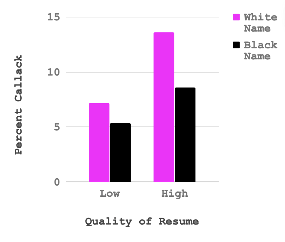
Data : Bertrand, M., & Mullainathan, S. (2004). Are Emily and Greg more employable than Lakisha and Jamal? A field experiment on labor market discrimination. American economic review, 94(4), 991-1013.
What is the relationship between resume quality and callback for white sounding names?
What is the relationship between resume quality and callback for black sounding names?
What is the difference in these slopes (is there an interaction effect?)
Frantz Fanon, Black Skin White Masks (1967) : “To speak means to be in a position to use a certain syntax, to grasp the morphology of this or that language, but it means above all to assume a culture, to support the weight of civilization…Every colonized people–in other words, every people in whose soul an inferiority complex has been created by the death and burial of its local cultural originality–finds itself face to face with the language of the civilizing nation; that is, with the culture of the mother country. The colonized is elevated above his jungle status in proportion to his adoption of the mother country’s cultural standards.”
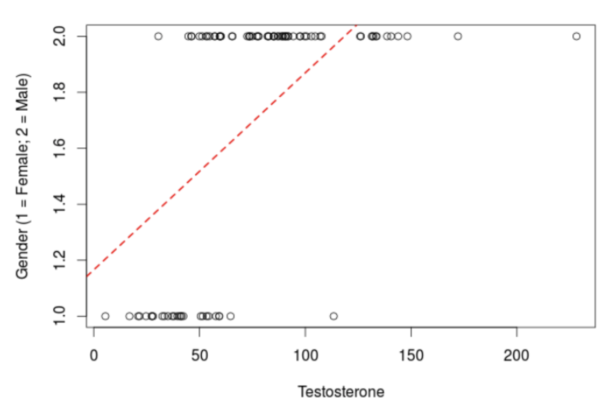
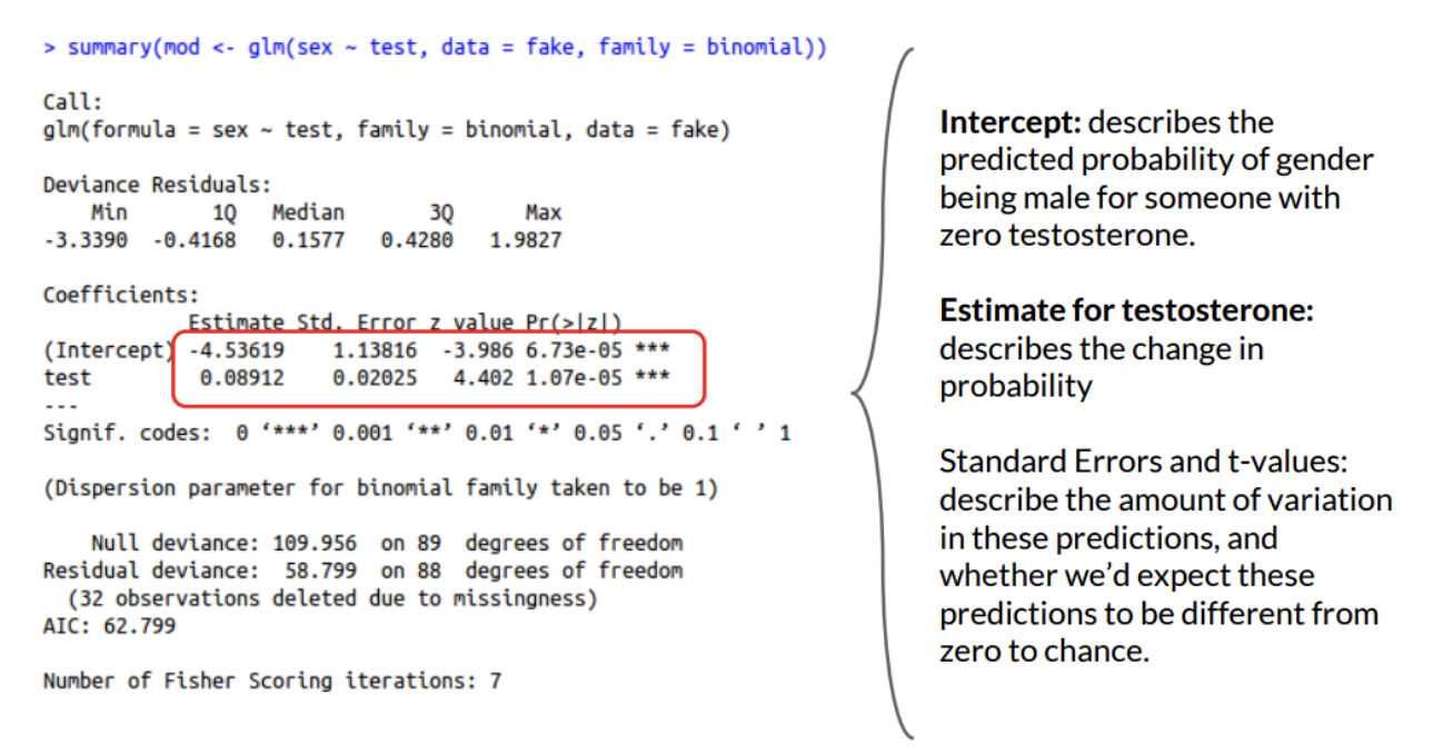
Generalized Linear Models (e.g., “Logistic Regression”)
Discussion : What do you observe about the relationship between testosterone and sex (as a DV)? Why is this model “wrong”??
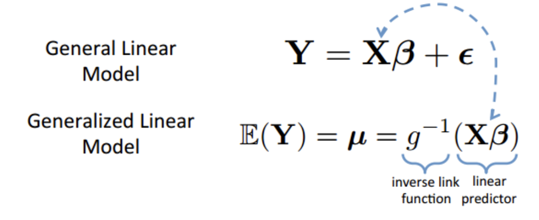
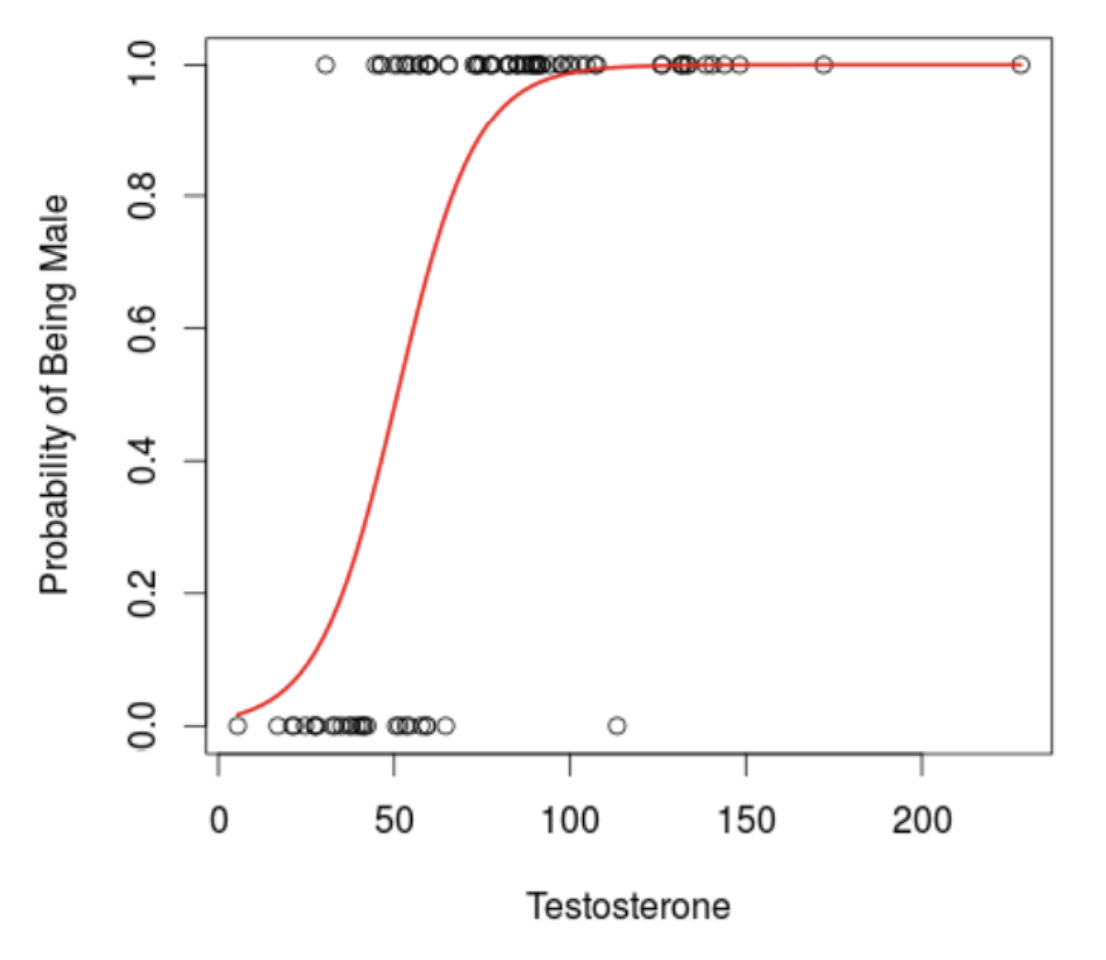
The Generalized Linear Model : Same Ideas (slope; intercept; error), but a “Link” Function that Transforms the Line to Fit Different Distributions.
Example : Defining a logistic regression (binomial distribution)
Multilevel Linear Models (e.g., HLM; MLM; dependent t-test)
Example : The Sleep Dataset (?sleep) : “Data which show the effect of two soporific drugs (increase in hours of sleep compared to control).”
Extra : increase in hours of sleep
Group : drug given (1 = control; 2 = drug)
ID : patient ID
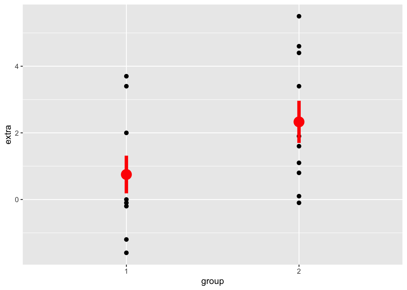
Sleep Data as a “General” Linear Model (a “Between Person” Study)
library(ggplot2)ggplot(sleep, aes(y = extra, x = group)) +geom_point(size=2) +stat_summary(fun.data=mean_se, color ='red', size =1.25, linewidth =2)
lmod <-lm(extra ~as.factor(group), data = sleep)summary(lmod)
Call:
lm(formula = extra ~ as.factor(group), data = sleep)

Residuals:
   Min     1Q Median     3Q    Max
-2.430 -1.305 -0.580  1.455  3.170

Coefficients:
                  Estimate Std. Error t value Pr(>|t|)
(Intercept)         0.7500     0.6004   1.249   0.2276
as.factor(group)2   1.5800     0.8491   1.861   0.0792 .
---
Signif. codes:  0 '***' 0.001 '**' 0.01 '*' 0.05 '.' 0.1 ' ' 1

Residual standard error: 1.899 on 18 degrees of freedom
Multiple R-squared:  0.1613,    Adjusted R-squared:  0.1147
F-statistic: 3.463 on 1 and 18 DF,  p-value: 0.07919
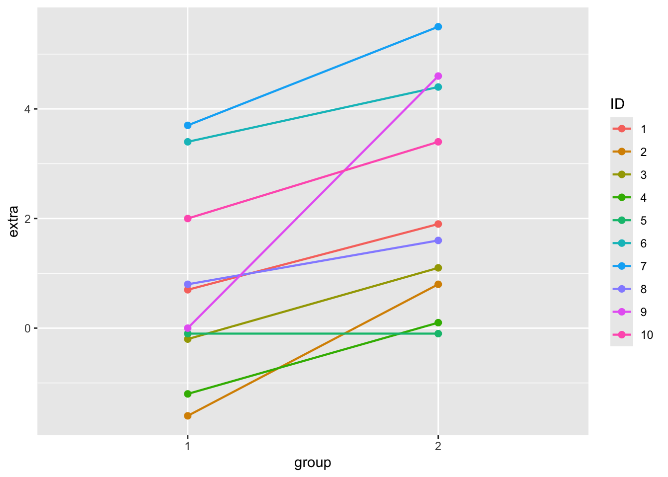
Sleep Data as a “Multilevel” Linear Model (a “Within-Person” Study). Many linear models! Look at the graph below. What’s going on? What do you observe? How might this help us understand the relationship between these two variables?
ggplot(sleep, aes(y = extra, x = group, color = ID)) +geom_point(size=2) +geom_line(aes(group = ID), linewidth =0.75)
What’s going on in the (random intercept) model. Still just one equation.
#install.packages("lme4")library(lme4)
Loading required package: Matrix
library(lmerTest)
Attaching package: 'lmerTest'
The following object is masked from 'package:lme4':

    lmer
The following object is masked from 'package:stats':

    step
library(Matrix)mlmod <-lmer(extra ~as.factor(group) + (1| ID), data = sleep)summary(mlmod)
Linear mixed model fit by REML. t-tests use Satterthwaite's method [
lmerModLmerTest]
Formula: extra ~ as.factor(group) + (1 | ID)
   Data: sleep

REML criterion at convergence: 70

Scaled residuals:
     Min       1Q   Median       3Q      Max
-1.63372 -0.34157  0.03346  0.31511  1.83859

Random effects:
 Groups   Name        Variance Std.Dev.
 ID       (Intercept) 2.8483   1.6877
 Residual             0.7564   0.8697
Number of obs: 20, groups:  ID, 10

Fixed effects:
                  Estimate Std. Error      df t value Pr(>|t|)
(Intercept)         0.7500     0.6004 11.0814   1.249  0.23735
as.factor(group)2   1.5800     0.3890  9.0000   4.062  0.00283 **
---
Signif. codes:  0 '***' 0.001 '**' 0.01 '*' 0.05 '.' 0.1 ' ' 1

Correlation of Fixed Effects:
            (Intr)
as.fctr(g)2 -0.324
Psych 102 (Honors Students Priority). You will need to advocate HARD for yourself to take this class.
Stat 133. Hear good things?
Sit in / Register for Psych 205 (Graduate Statistics). I taught this this semester; maybe again? IDK.
Practice The Thing You Want to Do!
RA —> Honors Thesis Pipeline. Psych 199 positions are posted on the psych website, but also do direct reach out to grad students who are involved in research that interests you.

 The Learning is Over; Would You Like to Learn More?