Quarto Power

Check-In : NHST Re-Review

#install.packages("jtools")
library(gplots)


Attaching package: 'gplots'

The following object is masked from 'package:stats':

    lowess

library(jtools)
library(car)

Loading required package: carData

mod1 <- lm(salary ~ yrs.service, data = Salaries)
mod2 <- lm(salary ~ sex, data = Salaries)
mod3 <- lm(yrs.service ~ sex, data = Salaries)
mod4 <- lm(salary ~ yrs.service + sex, data = Salaries)
export_summs(mod1, mod2, mod4)

	Model 1	Model 2	Model 3
(Intercept)	99974.65 ***	101002.41 ***	92356.95 ***
	(2416.61)	(4809.39)	(4740.19)
yrs.service	779.57 ***		747.61 ***
	(110.42)		(111.40)
sexMale		14088.01 **	9071.80
		(5064.58)	(4861.64)
N	397	397	397
R2	0.11	0.02	0.12
* p < 0.001; p < 0.01; * p < 0.05.

Power Tests

what’s the point, professor? (I’m tired.)

Power : the probability that you would “correctly” observe a “true” relationship between two variables that exists.
- goal : you want power to be HIGH. Power increases as…
  - the effect size increases : the bigger the difference, the more likely you’ll detect it.
  - your sample size increases : the more people, the less sampling error, and the easier it is to have confidence that any difference you found is not just chance.
  - you increase the threshold for rejecting the null hypothesis : if the probability
- assumptions : there is a true relationship; you have observed this relationship.
Reasons to Calculate Power :
- Post-Hoc Power : You did a study, and want to further contextualize your guess about how much sampling error influenced your results.
- Power Planning : You are planning to run a study, and want to know how many people to recruit to have the highest probability of observing the “true” effect (if it exists.)

a tour of null and alternative realities

Watch the lecture recording for a tour through these slides.

calculating in R (by hand)

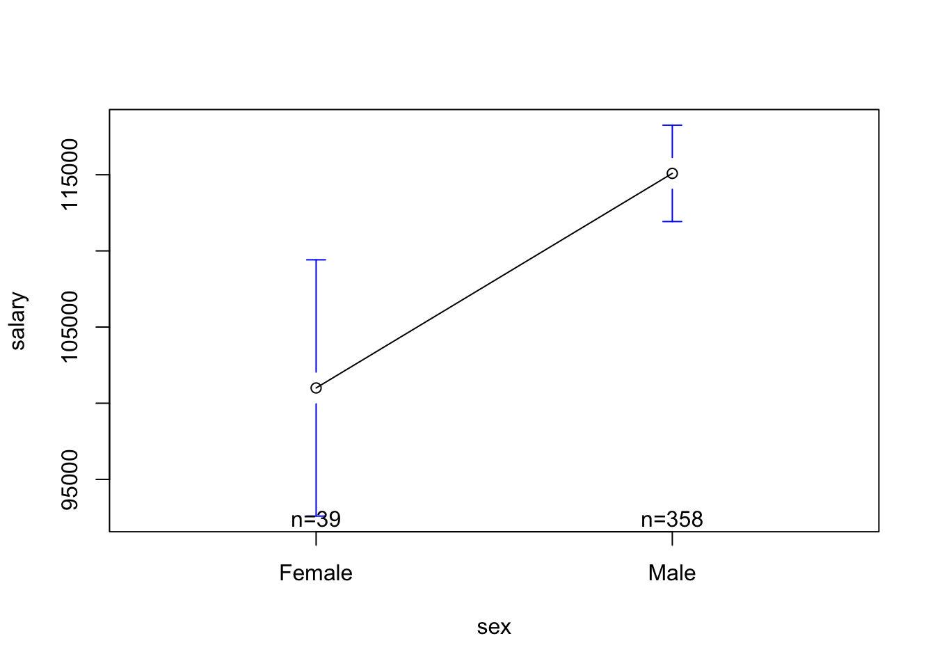
## The Model
plotmeans(salary ~ sex, data = Salaries)

mod2 <- lm(salary ~ sex, data = Salaries)
coef(mod2)

(Intercept)     sexMale 
  101002.41    14088.01

mod2 # a model object


Call:
lm(formula = salary ~ sex, data = Salaries)

Coefficients:
(Intercept)      sexMale  
     101002        14088

summary(mod2) # a function applied to the object


Call:
lm(formula = salary ~ sex, data = Salaries)

Residuals:
   Min     1Q Median     3Q    Max 
-57290 -23502  -6828  19710 116455 

Coefficients:
            Estimate Std. Error t value Pr(>|t|)    
(Intercept)   101002       4809  21.001  < 2e-16 ***
sexMale        14088       5065   2.782  0.00567 ** 
---
Signif. codes:  0 '***' 0.001 '**' 0.01 '*' 0.05 '.' 0.1 ' ' 1

Residual standard error: 30030 on 395 degrees of freedom
Multiple R-squared:  0.01921,   Adjusted R-squared:  0.01673 
F-statistic: 7.738 on 1 and 395 DF,  p-value: 0.005667

sm <- summary(mod2) # saving this as an object
objects(sm) # there is more inside.

 [1] "adj.r.squared" "aliased"       "call"          "coefficients" 
 [5] "cov.unscaled"  "df"            "fstatistic"    "r.squared"    
 [9] "residuals"     "sigma"         "terms"

sm$coefficients # tadaa

             Estimate Std. Error   t value     Pr(>|t|)
(Intercept) 101002.41   4809.386 21.001103 2.683482e-66
sexMale      14088.01   5064.579  2.781674 5.667107e-03

sm$coefficients[2,3] # our t-value

[1] 2.781674

mtval <- sm$coefficients[2,3]

qt(.975, df = 395) # t-distribution approaches the normal distribution (with a 95% Interval cutoff of 1.96....)

[1] 1.965988

mcut <- qt(.975, 395) # saving this cutoff value.

pt(mtval - mcut, df = 395) # our power.

[1] 0.7924144

calculating in R (a package)

# install.packages("pwr")
library(pwr)
summary(mod2)


Call:
lm(formula = salary ~ sex, data = Salaries)

Residuals:
   Min     1Q Median     3Q    Max 
-57290 -23502  -6828  19710 116455 

Coefficients:
            Estimate Std. Error t value Pr(>|t|)    
(Intercept)   101002       4809  21.001  < 2e-16 ***
sexMale        14088       5065   2.782  0.00567 ** 
---
Signif. codes:  0 '***' 0.001 '**' 0.01 '*' 0.05 '.' 0.1 ' ' 1

Residual standard error: 30030 on 395 degrees of freedom
Multiple R-squared:  0.01921,   Adjusted R-squared:  0.01673 
F-statistic: 7.738 on 1 and 395 DF,  p-value: 0.005667

nm <- nrow(mod2$model)
mr <- summary(mod2)$r.squared^.5
pwr.r.test(n = nm, r = mr) # similar to our calculation "by hand"


     approximate correlation power calculation (arctangh transformation) 

              n = 397
              r = 0.1386102
      sig.level = 0.05
          power = 0.7916982
    alternative = two.sided

ACTIVITY : calculate the power we had to detect the “independent” effect of sex on Salary, controlling for years of experience.

summary(mod4)


Call:
lm(formula = salary ~ yrs.service + sex, data = Salaries)

Residuals:
   Min     1Q Median     3Q    Max 
-81757 -20614  -3376  16779 101707 

Coefficients:
            Estimate Std. Error t value Pr(>|t|)    
(Intercept)  92356.9     4740.2  19.484  < 2e-16 ***
yrs.service    747.6      111.4   6.711 6.74e-11 ***
sexMale       9071.8     4861.6   1.866   0.0628 .  
---
Signif. codes:  0 '***' 0.001 '**' 0.01 '*' 0.05 '.' 0.1 ' ' 1

Residual standard error: 28490 on 394 degrees of freedom
Multiple R-squared:  0.1198,    Adjusted R-squared:  0.1154 
F-statistic: 26.82 on 2 and 394 DF,  p-value: 1.201e-11

Power Illustrated.

In lecture, professor likely did some scribbles on the whiteboard to illustrate power. One day, professor would like to find the time to record some more official videos illustrating power. However, he does currently not have this time. However, he did remember that - in 2018 - he had this time and thought thse videos might help. (What were you doing in 2018?? Let us know on Discord; and as always - reach out if you still have questions about power!!)

Recording #1 : Conceptual Example of Power
Recording #2 : Another Example. Couldn’t immediately track down the original data analyses these refer to, but the slope (b = .44) and other statistics come from a paper I had rejected in part because reviewers complained that I only replicated the main result in 4 out of 5 studies. (The paper was also a hot mess.) Bummer! But it was a cool phenomenon; I sadly never published on it for a variety of REASONS, but the truth got out eventually someone published a very clearly written, much better, and perfectly replicating paper (across six studies!) on it 8 years later. Ahhh, one thing off the to-do list!

Using Power to Estimate Sample Size.

As discussed in the lecture slides (see recording), power is a function of effect size, sample size, and the alpha level (alpha = the Type I error that the researcher sets). This means that you can use these functions to estimate the sample size you need for a given power (the convention is often 80%).

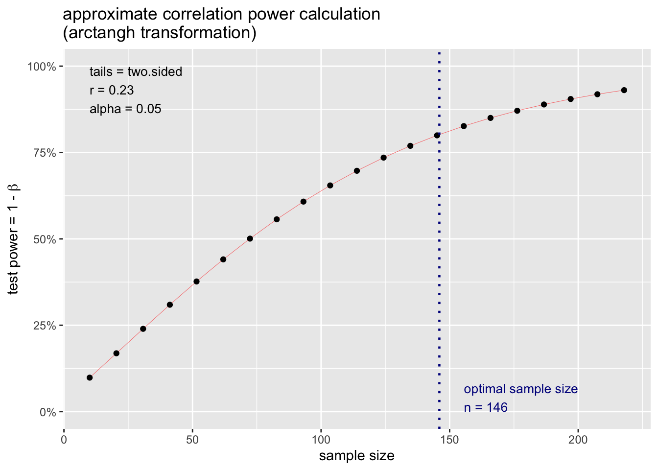
Let’s say I want to know what sample size I need to detect a slope of r = .23.

From the pwr package, I can define this effect, specifcy the power, type I error level, and whether I want to do a 1- or 2-tailed test.

pwr.r.test(r = .23, power = .80, alternative = "two.sided")


     approximate correlation power calculation (arctangh transformation) 

              n = 145.2367
              r = 0.23
      sig.level = 0.05
          power = 0.8
    alternative = two.sided

I can also plot the result of this output and see how power increases as a function of my sample size.

p.ex <- pwr.r.test(r = .23, power = .80, alternative = "two.sided")
plot(p.ex)

…but you don’t have to take my word for it. (More Resources)

The approach to power described above assumes a normally distribution of sampling error. This is a good starting place, but not all distributions are gaussian! Below are a few different methods to help you estimate power across a wide variety of types of data.

Here’s a nice overview of how to conduct sample size power analysis in R; it works through a few examples and discusses how to
This is a modern, thorough, and good overview of power, that also discusses ways to generate simulated data to estimate power..
Here’s another tutorial of an R package that works for a wide variety of different tests; many of which can be used when yout think the assumptions of linear regression are violated.
Let me know if you find other useful resources to help calcualte or conceptualize power!

Multiple Regression : More Regression

Labeling Changes

“Independent” Effect. The slope of the IV does not change when other variables are added to the model.
“Suppression” Effect. The slope of the IV gets stronger (in either direction) when other variables are added to the model.
“Mediation” Effect. The slope of the IV gets closer to zero when other variables are added to the model. Careful : “mediation” often implies some causal relationship, and it is very hard (/impossible?) to estimate causal relationships without experimental methods. Some links below that go deeper into this.

How Large a Change is Enough to Matter???

Is the difference in slope between Model 1 and Model 3 significant?

export_summs(mod1, mod2, mod4)

	Model 1	Model 2	Model 3
(Intercept)	99974.65 ***	101002.41 ***	92356.95 ***
	(2416.61)	(4809.39)	(4740.19)
yrs.service	779.57 ***		747.61 ***
	(110.42)		(111.40)
sexMale		14088.01 **	9071.80
		(5064.58)	(4861.64)
N	397	397	397
R2	0.11	0.02	0.12
* p < 0.001; p < 0.01; * p < 0.05.

bucket <- array()
for(i in c(1:1000)){
  sim <- Salaries[sample(1:nrow(Salaries), nrow(Salaries), replace = T),]
  xm1 <- lm(salary ~ sex, data = sim)
  xm2 <- lm(salary ~ sex + yrs.service, data = sim)
  bucket[i] <- coef(xm1)[2] - coef(xm2)[2]
}
sum(bucket > 0)

[1] 1000

Would You Like to Learn More?

The Difference Between “Significant” and “Not Significant” is not Itself Statistically Significant
A conceptual review of mediation, and tour through the ‘mediation’ package.
Preacher KJ, Hayes AF. Asymptotic and resampling strategies for assessing and comparing indirect effects in multiple mediator models. Behav Res Methods. 2008;40(3):879-891. doi:10.3758/BRM.40.3.879
A nice and recent summary of why caution is needed for mediation analysis.

Presentations

Multiple Regression : Moderation / Interaction Effects

Picture is worth…that’s right class…1000 words.

library(ggplot2)
library(ggthemes)
ggplot(data = Salaries, aes(x = yrs.service, y = salary, color = sex)) + 
  geom_point(size = .5, alpha = .3, position = "jitter") + 
  labs(title = "The Interaction Effect", x = "Years of Service", y = "Salary", color = "Sex") +
  geom_smooth(method = lm) + theme_apa()

`geom_smooth()` using formula = 'y ~ x'

Still just a linear model…

A linear model whose IVs must be standardized!!

mod5 <- lm(salary ~ yrs.service * sex, data = Salaries)
m5z <- scale_lm(mod5, scale.response = T) # 
m5z


Call:
lm(formula = salary ~ yrs.service * sex)

Coefficients:
        (Intercept)          yrs.service              sexMale  
           -0.09236              0.70305              0.12270  
yrs.service:sexMale  
           -0.40008

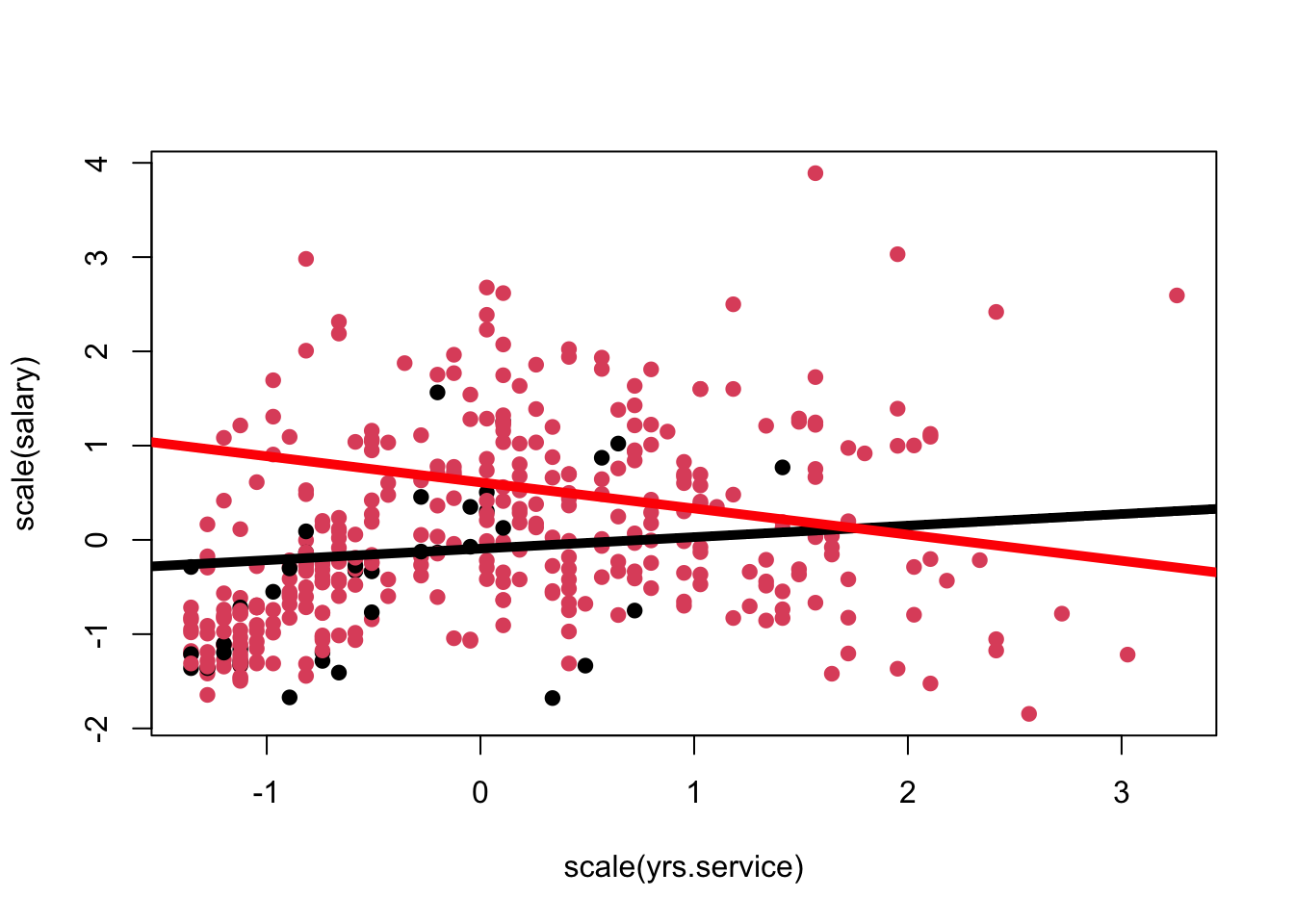
cf5 <- coef(m5z)
plot(scale(salary) ~ scale(yrs.service), col = sex, data = Salaries, pch = 19)
abline(a = cf5[1],
       b = cf5[3], 
       col = "black", lwd = 5) # line for females
abline(a = cf5[1] + cf5[2],
       b = cf5[3] + cf5[4], 
       col = "red", lwd = 5) # line for males

Reporting, and in a table.

export_summs(mod1, mod2, mod4, mod5)

	Model 1	Model 2	Model 3	Model 4
(Intercept)	99974.65 ***	101002.41 ***	92356.95 ***	82068.51 ***
	(2416.61)	(4809.39)	(4740.19)	(7568.72)
yrs.service	779.57 ***		747.61 ***	1637.30 **
	(110.42)		(111.40)	(523.03)
sexMale		14088.01 **	9071.80	20128.63 *
		(5064.58)	(4861.64)	(7991.14)
yrs.service:sexMale				-931.74
				(535.24)
N	397	397	397	397
R2	0.11	0.02	0.12	0.13
* p < 0.001; p < 0.01; * p < 0.05.

Would You Like To Learn More?

As always, let me know if you find great resources :)

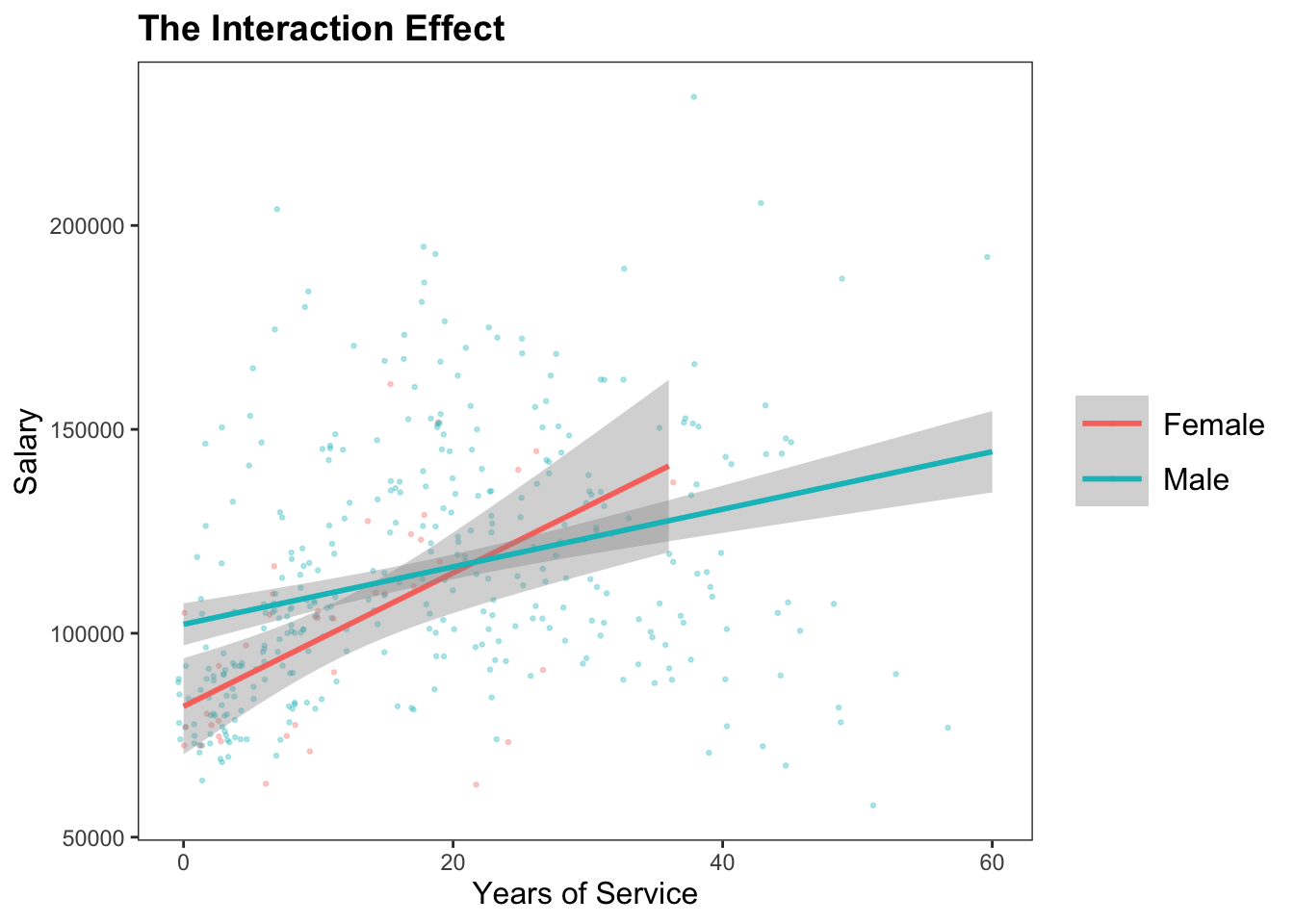
The Interactions Package. The author of jtools has made what looks like a super clean way to graph interaction effects in R, using ggplot2.
Visualization Tutorials. Other, more cumbersome methods of plotting interaction effects exist!

It’s Project Time

Find a buddy : someone who you haven’t spoken to