Look at the regression output in the lecture document to answer these questions. You will need to click through the different tabs to view all three models (and Model 1 regression diagnostic).
The study is described as the following : The 2008-09 nine-month academic salary for Assistant Professors, Associate Professors and Professors in a college in the U.S. The data were collected as part of the on-going effort of the college’s administration to monitor salary differences between male and female faculty members.”
salary : the salary of the professor, in cold, hard, US American Dollars.
yrs.service : the years of service the professor had at the college.
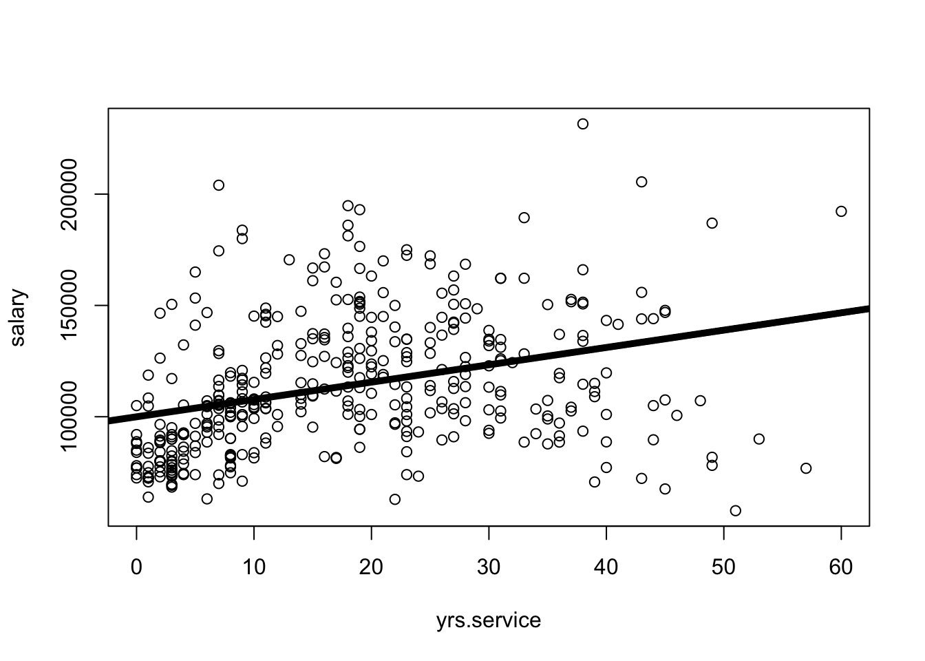
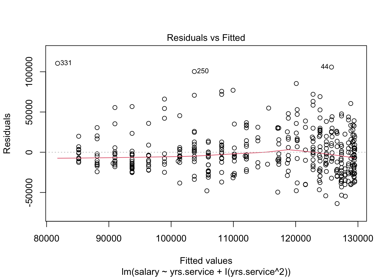
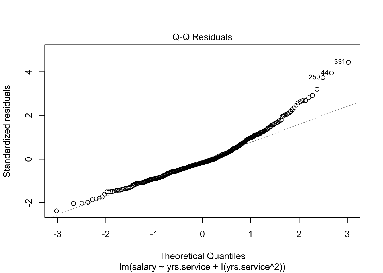
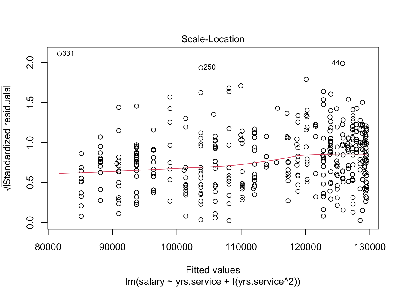
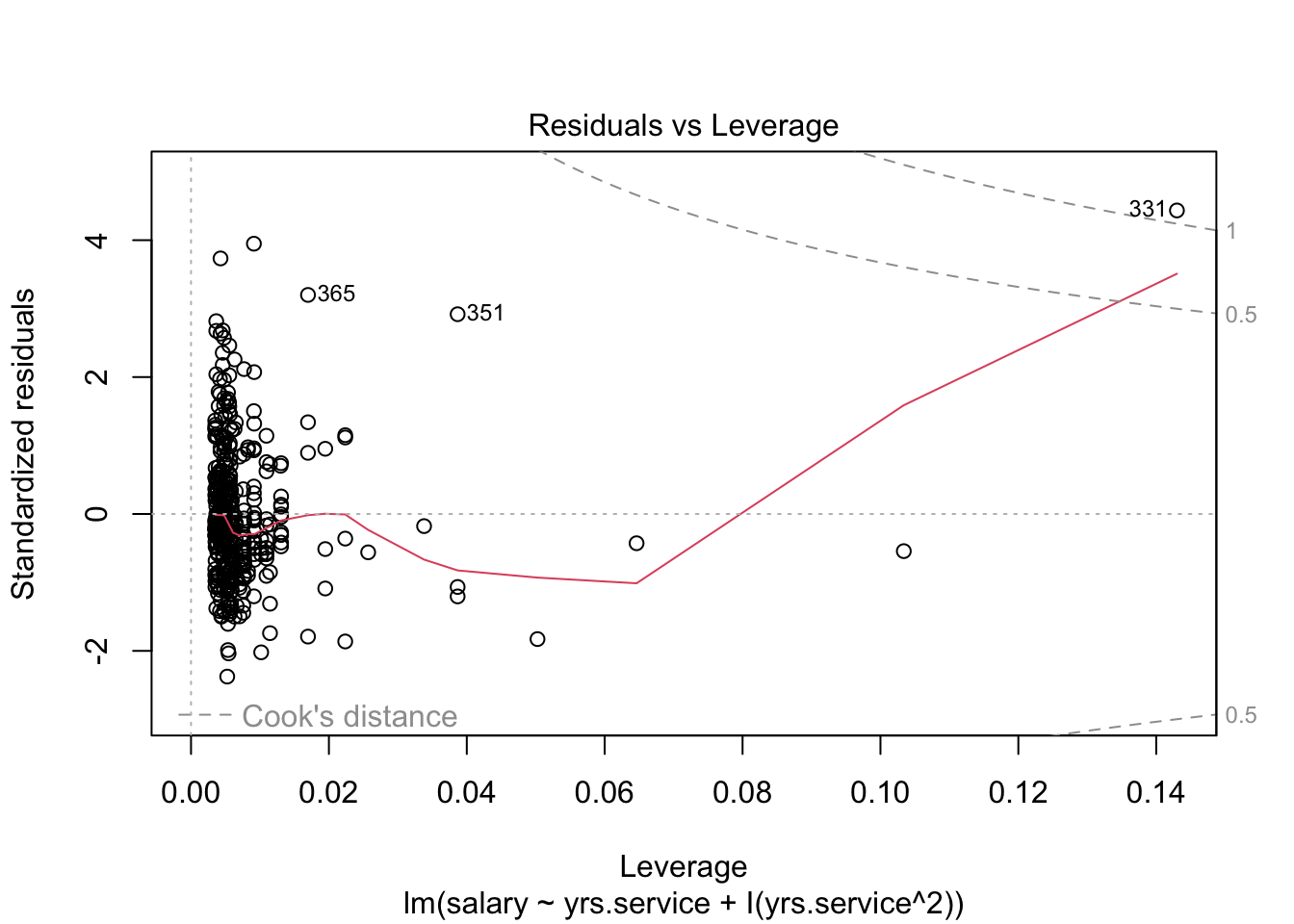
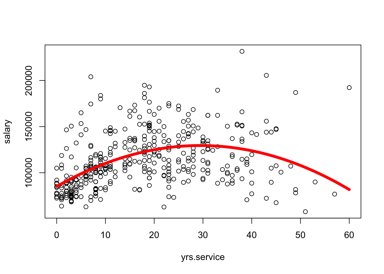
fake.dat <-data.frame(yrs.service =seq(min(Salaries$yrs.service), max(Salaries$yrs.service), length.out =100))pred.dat <-predict(mod1x, fake.dat)plot(salary ~ yrs.service, data = Salaries)lines(fake.dat$yrs.service, pred.dat, col ="red", lwd =5)
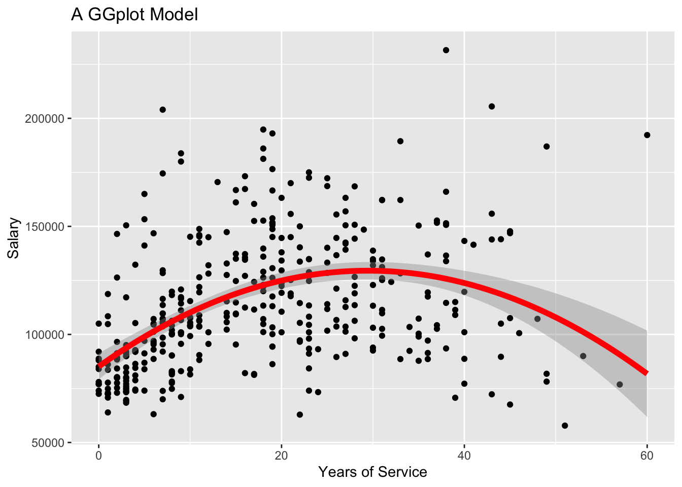
library(ggplot2)library(ggthemes)ggplot(data = Salaries, aes(x = yrs.service, y = salary)) +geom_point() +geom_smooth(method ="lm", formula = y ~poly(x, 2, raw =TRUE), color ="red", se =TRUE,linewidth =2) +labs(title ="A GGplot Model",x ="Years of Service",y ="Salary")
Did this change make things better??
What are some ways we could answer this question???
R^2 goes up!!!
the quadratic term was significant!!!!
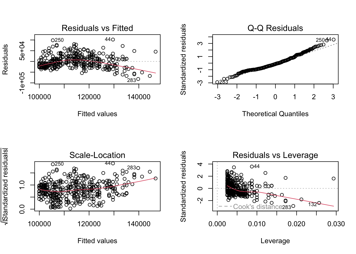
there’s less heteroscedasticity (one of the assumptions of regresssion in those plots!!!)
Account for multiple variables to help predict and explain the DV.
Control for the effect of on IV on the relationship between another IV and the DV.
Compare unique effects of each IV on the DV. See how the slope of one IV compares to the slope of another IV. (Need to standardize your variables, to make sure that they are all on the same scale.)
NEXT WEEK : Interaction Effects!!! See how the relationship between one IV and the DV changes depending on another IV.
In Practice.
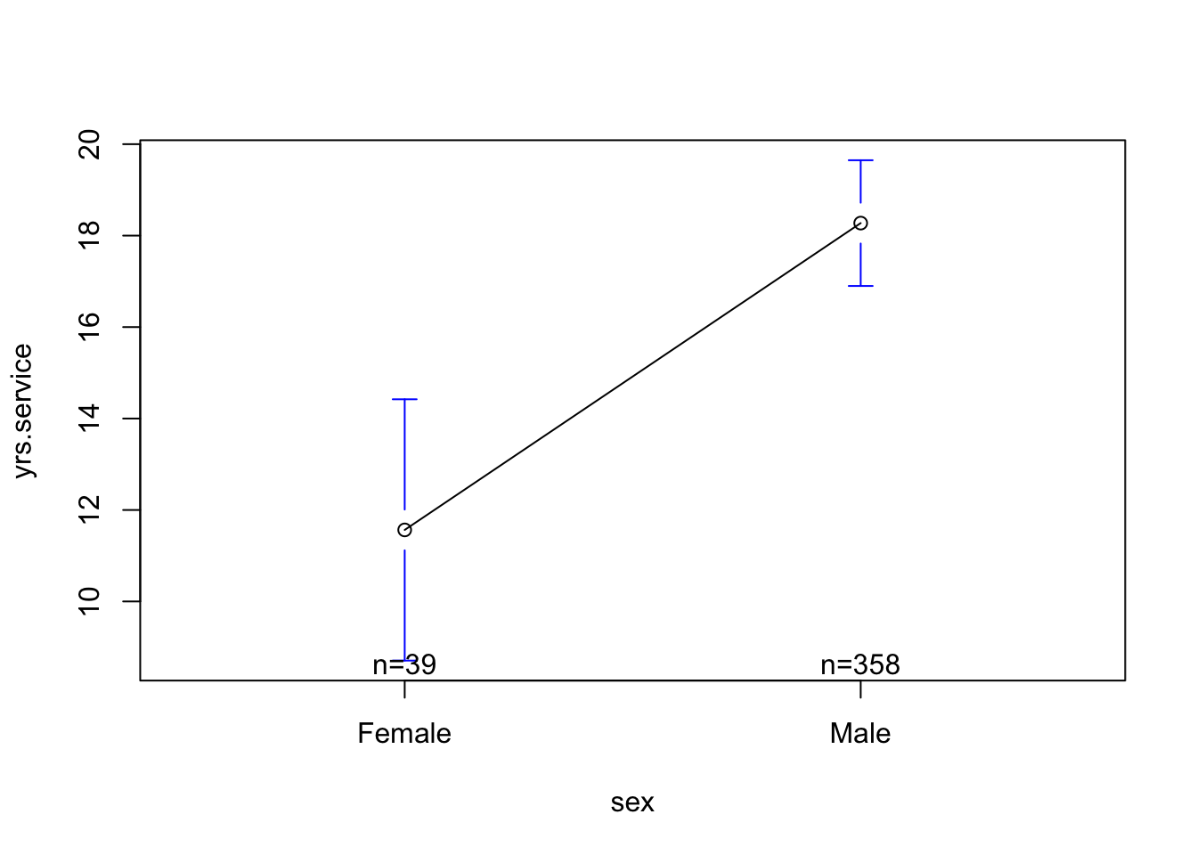
mod1 <-lm(salary ~ yrs.service, data = Salaries)mod2 <-lm(salary ~ sex, data = Salaries)mod3 <-lm(yrs.service ~ sex, data = Salaries)mod4 <-lm(salary ~ yrs.service + sex, data = Salaries)summary(mod4)
Call:
lm(formula = salary ~ yrs.service + sex, data = Salaries)
Residuals:
Min 1Q Median 3Q Max
-81757 -20614 -3376 16779 101707
Coefficients:
Estimate Std. Error t value Pr(>|t|)
(Intercept) 92356.9 4740.2 19.484 < 2e-16 ***
yrs.service 747.6 111.4 6.711 6.74e-11 ***
sexMale 9071.8 4861.6 1.866 0.0628 .
---
Signif. codes: 0 '***' 0.001 '**' 0.01 '*' 0.05 '.' 0.1 ' ' 1
Residual standard error: 28490 on 394 degrees of freedom
Multiple R-squared: 0.1198, Adjusted R-squared: 0.1154
F-statistic: 26.82 on 2 and 394 DF, p-value: 1.201e-11
Discussion : What Do You Observe Changing About the Model???? What’s the same???
the effect of gender :
males STILL make more than females (b = 9071), even when accounting for years of service.
this effect went down in size (it was 14,088 in the bivariate model) = “partial mediation” (CAREFUL!!!!)
with this lower efffect size, we are LESS confidient that the difference is not just random sampling (p-value for gender difference = .06 = is no longer significant)
the effect of yrs.service :
we still see a positive relationship: more years of service = more $ (b = $747.6 for every extra year or service.)
this effect also went down a little (was b = 779.6 in the bivariate model (model 1).)
the effect is still significant.
the model : our predictions are pretty much the same…..but a little higher (R^2 went from .11 to .12.)
QUESTIONS WE HAVE :
what’s going on with F-TEST.
how does the model actually account for the co-variation / unique effects???
BREAK TIME : MEET BACK AT 12:57 PM THANKS!
Reporting Effects in a Regression Table
Table 1. Unstandardized Regression Coefficients; Predicting Salary from Years of Service and Sex.
Model 1
Model 2
Model 3
Intercept
99974
101002
92356
Years Service
779.6 **
—-
747.6 **
Sex
—
14088 **
9071 (+)
\(R^2\)
.11
.02
.12
Or, using a fun R package to do this.
library(jtools)export_summs(mod1, mod2, mod4)
Model 1
Model 2
Model 3
(Intercept)
99974.65 ***
101002.41 ***
92356.95 ***
(2416.61)
(4809.39)
(4740.19)
yrs.service
779.57 ***
747.61 ***
(110.42)
(111.40)
sexMale
14088.01 **
9071.80
(5064.58)
(4861.64)
N
397
397
397
R2
0.11
0.02
0.12
*** p < 0.001; ** p < 0.01; * p < 0.05.
?export_summslibrary(sjPlot)
Install package "strengejacke" from GitHub (`devtools::install_github("strengejacke/strengejacke")`) to load all sj-packages at once!
tab_model(mod1, mod2, mod4)
salary
salary
salary
Predictors
Estimates
CI
p
Estimates
CI
p
Estimates
CI
p
(Intercept)
99974.65
95223.64 – 104725.67
<0.001
101002.41
91547.22 – 110457.60
<0.001
92356.95
83037.72 – 101676.17
<0.001
yrs service
779.57
562.49 – 996.65
<0.001
747.61
528.61 – 966.62
<0.001
sex [Male]
14088.01
4131.11 – 24044.91
0.006
9071.80
-486.21 – 18629.81
0.063
Observations
397
397
397
R2 / R2 adjusted
0.112 / 0.110
0.019 / 0.017
0.120 / 0.115
Multiple Regression : Visualized in Multi-Dimensional Space!
The code below won’t run in quarto, and may not work on your comptuer; for teaching purposes!
#install.packages('rgl')#install.packages('car')library(car)library(rgl)scatter3d(as.numeric(Salaries$sex), # IV1 - must be numeric (if not already) Salaries$salary, # DV Salaries$yrs.service) # IV2 - must be numeric (if not already)
mod4 <-lm(salary ~ yrs.service + sex, data = Salaries)summary(mod4)
Call:
lm(formula = salary ~ yrs.service + sex, data = Salaries)
Residuals:
Min 1Q Median 3Q Max
-81757 -20614 -3376 16779 101707
Coefficients:
Estimate Std. Error t value Pr(>|t|)
(Intercept) 92356.9 4740.2 19.484 < 2e-16 ***
yrs.service 747.6 111.4 6.711 6.74e-11 ***
sexMale 9071.8 4861.6 1.866 0.0628 .
---
Signif. codes: 0 '***' 0.001 '**' 0.01 '*' 0.05 '.' 0.1 ' ' 1
Residual standard error: 28490 on 394 degrees of freedom
Multiple R-squared: 0.1198, Adjusted R-squared: 0.1154
F-statistic: 26.82 on 2 and 394 DF, p-value: 1.201e-11
It’s nice to organize your slopes and results using a regression table. R can make these for you.
library(jtools)export_summs(mod1, mod2, mod4)
Model 1
Model 2
Model 3
(Intercept)
99974.65 ***
101002.41 ***
92356.95 ***
(2416.61)
(4809.39)
(4740.19)
yrs.service
779.57 ***
747.61 ***
(110.42)
(111.40)
sexMale
14088.01 **
9071.80
(5064.58)
(4861.64)
N
397
397
397
R2
0.11
0.02
0.12
*** p < 0.001; ** p < 0.01; * p < 0.05.
Hey, Professor. Some of us are applying to graduate school and could use some guidance or help?
Not Code. Personal Statements, Professor!!!!
Start with what you’re doing at Cal –> why you are ready to begin at the specific school (and advisor(s)) you’re applying to.
applying to work with specific people - focus on a primary, but list a few others.
check website (or e-mail) before to see if they are accepting. If you e-mail….
1-2 sentences about who you are, working at Cal with professor (HT advisor) on a project related to (connect to their interests; flatter them).
I’m super interested in your work on BLAH BLAH BLAH.
Wondering if you are accepting new students. Also interested in OTHER TOPICS, and possibly working with Drs. SOSO on other projects as I progress through the program. I know programs differ in the extent to whcih they encourage or allow studnets to work with multiple advisors, and wondered what your perspective was.
Thanks for your time!
Outline of Your Statement
Intro (very brief) : who you are, and a brief overview of some of the skills / accomplishments / interests that demonstrate YOU READY to be a grad student.
Middle Parts : Your Past Experiences.
The Point : give specific and clear examples of the work you did. Explain how this demonstrates more broad skills (e.g., intellect and work ethic, passion for psychology, resilience,) And then connect these skills to the work you might do as a grad student.
Some ideas : classes you took, work you did as an RA, honors thesis project, attending conferences, mentoring, supervising.
Example : “Took stats classes” –> “Learned how to use the program R to clean data, define linear models, estimate sampling error using bootstrap methods, critically evaluate graphs….etc. In grad school, I’m excited to….take more advanced stats classes? work with existing datasets the lab might have?? Just connect to your future! Connect this work to what you might do in graduate school. Was it related to the kinds of topics you might want to study in grad school? If so, cool! Can explain how they prepare you for the kinds of work you mgiht want to do, then go more specifically into that and those research interests. If not related, still talk about the broad skills.
Example : “I was a research assistant for X lab.” [Cool, but incomplete!!!] —> BETTER : I was a research assistant for X lab, where I worked on a project related to (PROJECT TOPIC GOES HERE.) In this role, I helped designed study materials, worked closely with the researchers to develop participant recruitment strategies, helped run the study, and attended regular lab meetings where. These experiences demonstrate….
Final Part : Your specific research interests / the school you are applying to.
you are applying to work with a specific advisor (or maybe a few), so connect your own interests to those that others are doing at the school.
great to have broad interests and not be 100% locked into an idea, but also good to show that you have specific ideas about what you want to do.
“I’m interested in BLAH BLAH. At SPECIFIC SCHOOL GO HERE, I hope to work with Dr. BLAH BLAH on studies related to BLAH. I’m also really interested in learning more about Drs. BLAH and BLAHs work….”
Other things to include :
coursework / areas of specialty this program has.
things related to the community you are interested in working with (e.g., are they in an urban setting that might work with specific populations?)
Power Tests
what’s the point, professor? (I’m tired.)
Power : the probability that you would “correctly” observe a “true” relationship between two variables that exists.
goal : you want power to be HIGH. Power increases as…
the effect size increases : the bigger the difference, the more likely you’ll detect it.
your sample size increases : the more people, the less sampling error, and the easier it is to have confidence that any difference you found is not just chance.
you increase the threshold for rejecting the null hypothesis : if the probability
assumptions : there is a true relationship; you have observed this relationship.
Reasons to Calculate Power :
Post-Hoc Power : You did a study, and want to further contextualize your guess about how much sampling error influenced your results.
Power Planning : You are planning to run a study, and want to know how many people to recruit to have the highest probability of observing the “true” effect (if it exists.)
a tour of null and alternative realities
Watch the lecture recording for a tour through these slides.
calculating in R (by hand)
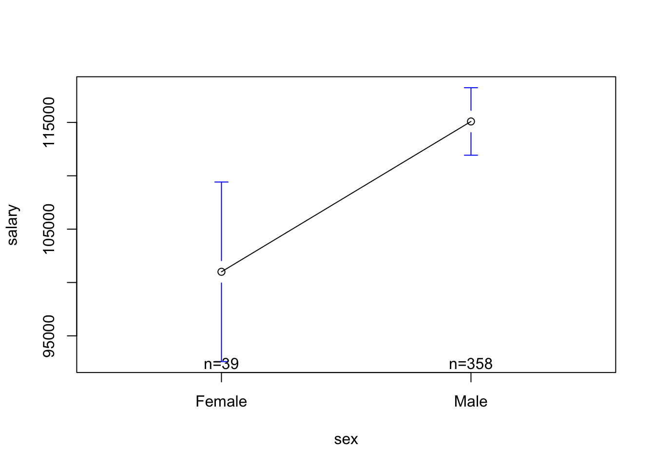
## The Modelplotmeans(salary ~ sex, data = Salaries)
mod2 <-lm(salary ~ sex, data = Salaries)coef(mod2)
Estimate Std. Error t value Pr(>|t|)
(Intercept) 101002.41 4809.386 21.001103 2.683482e-66
sexMale 14088.01 5064.579 2.781674 5.667107e-03
sm$coefficients[2,3] # our t-value
[1] 2.781674
mtval <- sm$coefficients[2,3]qt(.975, df =147) # t-distribution approaches the normal distribution (with a 95% Interval cutoff of 1.96....) but we are not quite there.
[1] 1.976233
mcut <-qt(.975, 147) # t-distribution approaches the normal distribution (with a 95% Interval cutoff of 1.96....) but we are not quite there.pt(mtval - mcut, df =147) # our power.
Call:
lm(formula = salary ~ sex, data = Salaries)

Residuals:
   Min     1Q Median     3Q    Max
-57290 -23502  -6828  19710 116455

Coefficients:
            Estimate Std. Error t value Pr(>|t|)
(Intercept)   101002       4809  21.001  < 2e-16 ***
sexMale        14088       5065   2.782  0.00567 **
---
Signif. codes:  0 '***' 0.001 '**' 0.01 '*' 0.05 '.' 0.1 ' ' 1

Residual standard error: 30030 on 395 degrees of freedom
Multiple R-squared:  0.01921,   Adjusted R-squared:  0.01673
F-statistic: 7.738 on 1 and 395 DF,  p-value: 0.005667
nm <-nrow(mod2$model)mr <-summary(mod2)$r.squared^.5pwr.r.test(n = nm, r = mr) # similar to our calculation "by hand"
     approximate correlation power calculation (arctangh transformation)

              n = 397
              r = 0.1386102
      sig.level = 0.05
          power = 0.7916982
    alternative = two.sided
ACTIVITY : calculate the power we had to detect the “independent” effect of sex on Salary, controlling for years of experience.
Power Illustrated.
In lecture, professor likely did some scribbles on the whiteboard to illustrate power. One day, professor would like to find the time to record some more official videos illustrating power. However, he does currently not have this time. However, he did remember that - in 2018 - he had this time and thought thse videos might help. (What were you doing in 2018?? Let us know on Discord; and as always - reach out if you still have questions about power!!)
Recording #2 : Another Example. Couldn’t immediately track down the original data analyses these refer to, but the slope (b = .44) and other statistics come from a paper I had rejected in part because reviewers complained that I only replicated the main result in 4 out of 5 studies. (The paper was also a hot mess.) Bummer! But it was a cool phenomenon; I sadly never published on it for a variety of REASONS, but the truth got out eventually someone published a very clearly written, much better, and perfectly replicating paper (across six studies!) on it 8 years later. Ahhh, one thing off the to-do list!
Using Power to Estimate Sample Size.
As discussed in the lecture slides (see recording), power is a function of effect size, sample size, and the alpha level (alpha = the Type I error that the researcher sets). This means that you can use these functions to estimate the sample size you need for a given power (the convention is often 80%).
Let’s say I want to know what sample size I need to detect a slope of r = .23.
From the pwr package, I can define this effect, specifcy the power, type I error level, and whether I want to do a 1- or 2-tailed test.
pwr.r.test(r = .23, power = .80, alternative ="two.sided")
     approximate correlation power calculation (arctangh transformation)

              n = 145.2367
              r = 0.23
      sig.level = 0.05
          power = 0.8
    alternative = two.sided
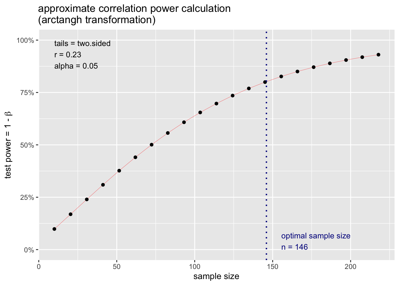
I can also plot the result of this output and see how power increases as a function of my sample size.
p.ex <-pwr.r.test(r = .23, power = .80, alternative ="two.sided")plot(p.ex)
…but you don’t have to take my word for it. (More Resources)
The approach to power described above assumes a normally distribution of sampling error. This is a good starting place, but not all distributions are gaussian! Below are a few different methods to help you estimate power across a wide variety of types of data.