Talking to your advisors / graduate students / TAs (/my old dissertation data?)
Other sources / ideas?
Brain Exam pushed back a week.
Comments on the Mid-Semester Evaluation
ideas for changes
“…find ways to have more class participation in the presentations so we can really get into the topics and have a communal sense of the class, but thats not something the professor can control so I think its good as is.”
“…dive more into the statistics itself so i have some theoretical background for the tests im doing (for example, our method for our thesis was due yesterday, and i was struggling to understand how to apply LME to my neural time series data..”
“…I think having some moment when there’s time to pause… it doesn’t have to be a 2-3 min pause, just like 20 sec so I can write the code as fast as the professor does.”
other comments :
“I’m still a little confused about data cleaning and when we should really take out data; how much is okay to remove from the dataset.”
“How are the article presentations supposed to help us?”
“Honors has been very stressful… but its ok.”
LAST TIME, ON METHODS IN PSYCHOLOGY….
We Found a Model
library(psych)library(gplots)
Attaching package: 'gplots'
The following object is masked from 'package:stats':

    lowess
d <-read.csv("~/Dropbox/!GRADSTATS/gradlab/Exams/objectivityposted.csv", stringsAsFactors = T)names(d)
I Asked Y’all To Do Some Interpretation of the Regression Assumptions.
Professor answers to the regression assumptions typed out below.
Validity. Were the data measured and collected in a valid way? I’d have to trust the researchers’ methods for getting these data, but feel like power words scraped by a comptuer program might have some validity issues, since it’s likely the algorithm the researchers are using (LIWC, from Pennebaker) isn’t really taking into full context (e.g., “not a strong relationship” would show as 1 power word.) Think it might also be hard to measure the author race, tho there’s always some error in measurement, so the question is whether the error is so biased that it skews the results, which is hard to say!
Reliability. Were the data measured with high reliability? Hmm, we don’t have a way to assess the reliability of these measures, since they are all single item ratings. Reliability is about repeatability, so I might want to check that the computer did its job right by having an unpaid RA working for that valuable experience manually count the power words, or maybe have a few RAs do some of the computer work and confirm there’s consistency between their responses. This is often something researchers do; will talk about other methods of estimating reliability later this semester. Another form of reliability - not examined here - would be to see whehter this trend holds up across other scientific disciplines.
Independence. Does one data point give you any information about another individual’s data point? (if yes, then not independent.) Ah, here is a violated assumption. The data are not technically independent - an author could have written multiple papers and their writing style for one article might influence their writing in another. Later, we will learn how to model this dependence in the data. I don’t think it’s super strong here / influnencing the results that much, but will be good to confirm. (And the authors mention in the paper they controlled for some of these effects with a multilevel linear model.)
Linearity. Are the predicted values of Y based on a constant and linear relationship with X? Time for some regression diagnostic plots! To run these, you plot the model object : plot(mod). Many of y’all have probably done this accidentally, but now its time to use this intentionally.
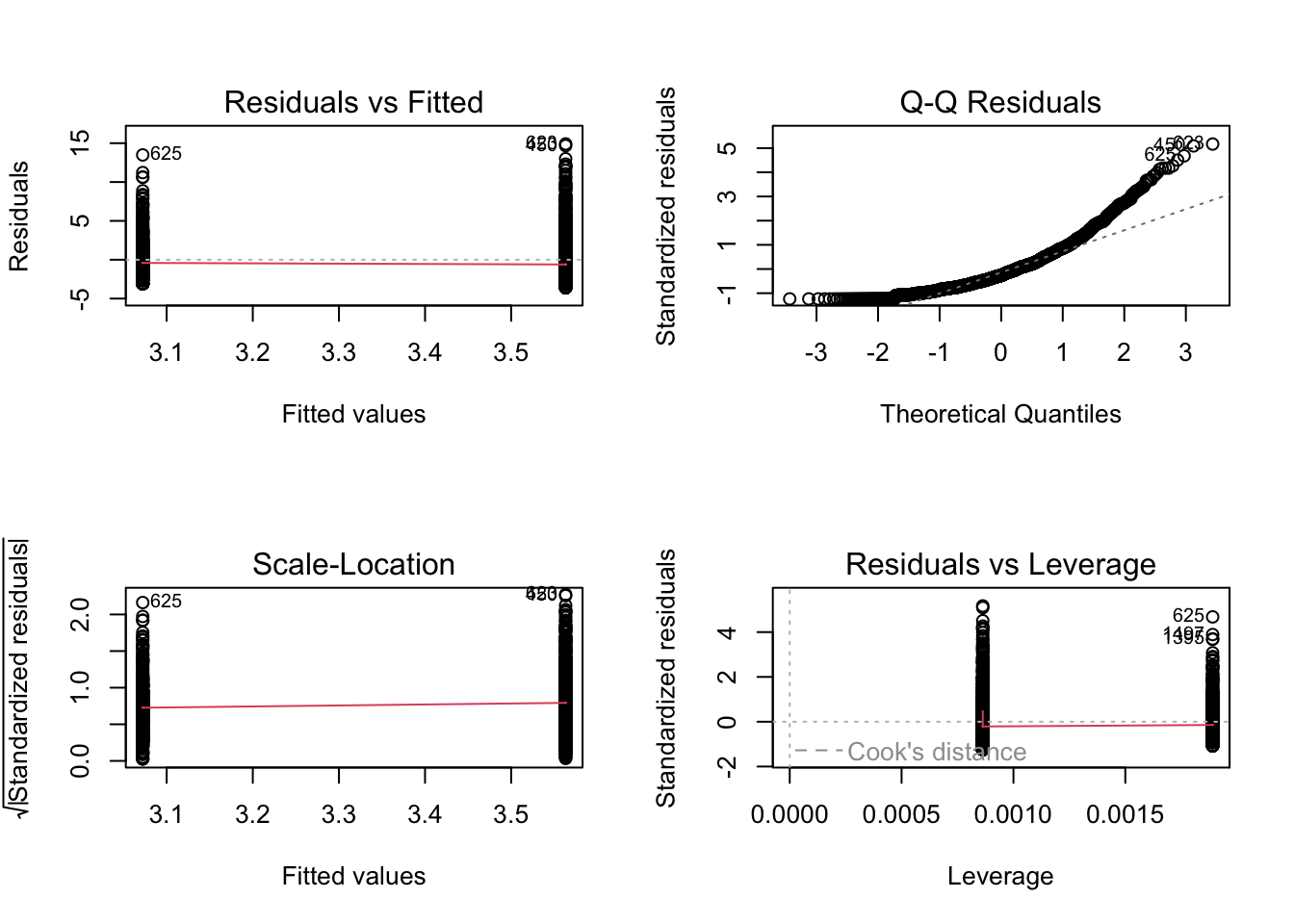
par(mfrow =c(2,2)) # splitting the graphics window into a 2x2 grid so we can see all four diagnostic plots.plot(mod) # the diagnostic plots.
You can read more about what these plots are doing in last week’s lecture notes, but the basic idea is you want to see constant variation in the distribution of the residuals (errors in our predictions), and each of these graphs tries to illustrate the residuals in some novel way.
I’m seeing some non-balanced graphs in the plots…for example, the residual vs. fitted graph below shows that my predicted values of power words for both groups (the authors of color on the left and white authors on the right) have more residuals far above the line than below. This is due to the highly-skewed data in power words, and I can see some of these patterns in the other graphs (e.g., in the Q-Q Residual plots where our actual residuals are much higher on the extreme ends than we might predict for a normal curve.) To fix this, I would probably apply some non-linear transformation to our DV to reduce the amount of skew.
Heteroscedasticity. Is there constant variation in the residuals across the fitted values? Again, there is non-constant variation in the residuals across the fitted values. I expect this to improve when we apply the non-linear transformation to the DV in our model. And maybe account for some of that non-Independence. I’m not super concerned about the individuals exerting leverage - they look far away, but looking at my original model I notice a) there’s a lot of data, so outliers won’t have as much influence and b) these leverage statistics are small in value. You can read more about how leverage is calculated (see Lecture 5 notes), but Cook’s Distance calculates a threshold for an “appropriate” amount of leverage, and these data fall within that range.
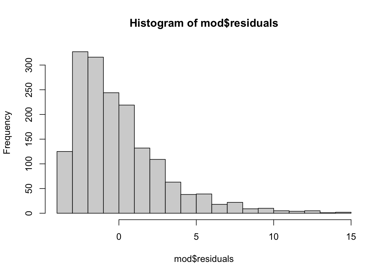
Normality of Errors. Are the residuals in the model normally distributed? The residuals are not normal; doing a non-linear transformation of the DV will improve the normality of this.
hist(mod$residuals, breaks =20)
Transforming Regression Coefficients.
Sometimes, we need (or want) to change the structure of our data to address violated assumptions, or change the units and our interpretation.
Numeric Transformations
RECAP : Linear Transformations
Linear transformations change the units, but do not change the position of the individual data points. Below are a few new examples of linear transformations, hanging out with our old friend the z-score.
“Percent of Maximum Possible” (POMP)
equation and example :\(100*\frac{x}{max(x)}\)
what it does : stretches out the scale of a variable, so 0 = people who scored the lowest and 100 = people who scored the highest.
when to use : maybe helps people conceptualize likert scales (but also can exaggerate effects; e.g., a 1-5 scale turns into a 0-100 scale, which makes the slope seem larger)
Mean-Centering :
equation and example :\(x_i - mean(x)\)
what it does : redefines individual scores in terms of how far above or below the mean they are.
when to use : you want zero to be defined as the average of the variable, but do not want to lose the units of measurement (e.g., a zero for heart rate BMP is dead, but zero of mean-centered BMP is the average heart rate)
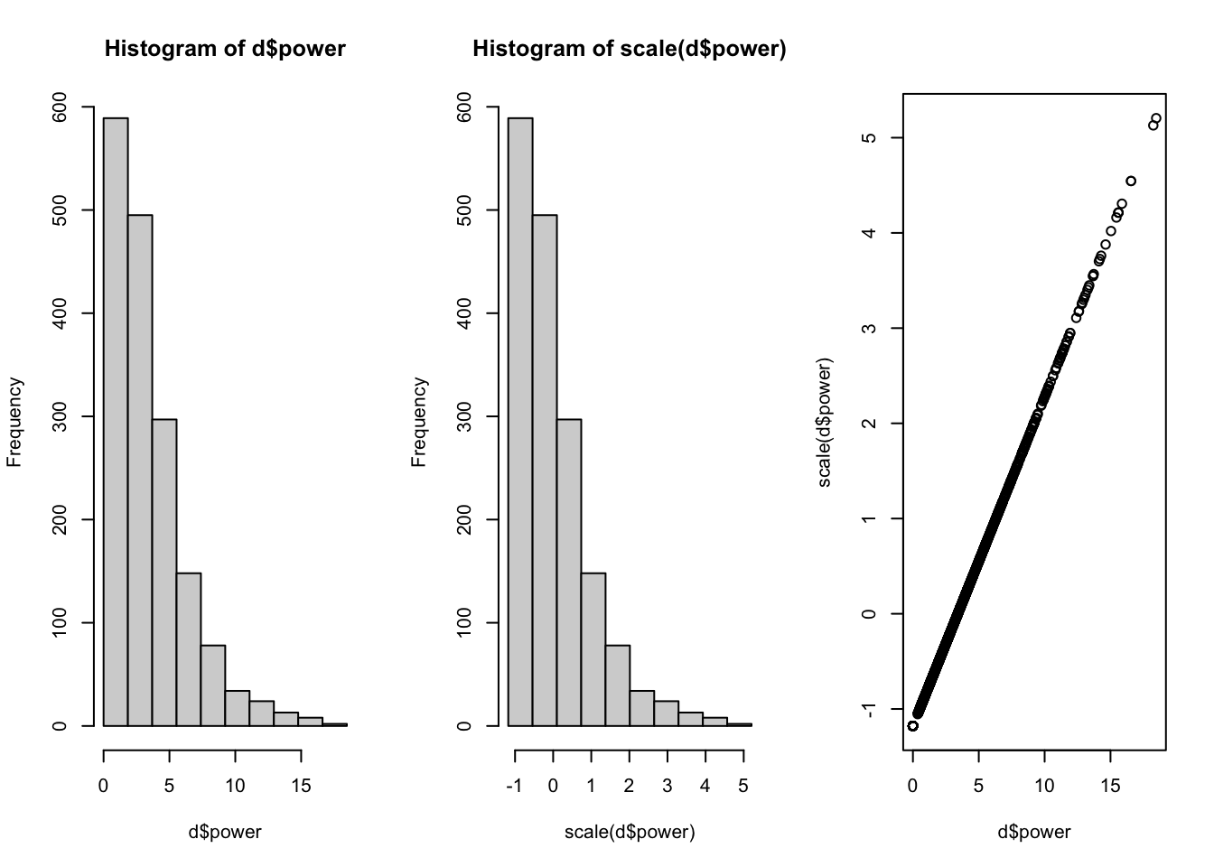
Z-Score. We already discussed and defined this in a previous lecture.
equation and example :\(z = \frac{x_i - mean(x)}{sd(x)}\)
what it does : redefines individual scores in terms of how far above or below the mean they are, relative to the standard deviation (so, how different from the mean a score is, but contextualizing this difference in terms of how .)
when to use : you want to remove the units from your measure (and model).
Non-Linear Transformations : Log; Square-Root; Exp; etc.
Non-linear transformations radically alter the shape of your distribution, and the position of your individual data (relative to each other). These transformations are most often used to make non-normal distributions look more normal.
Log Transformation.
equation and example : see the table below. Logs are confusing (I think.)
what it does : compresses the scale of a variable (the log takes a number, and transforms it to be the exponent which a specific base must be raised to create the number).
when to use : address heteroscedasticity by normalizing positively skewed data (e.g., count data; data with a floor effect); natural log is used in growth models.
Transformation in R
Base (b)
Formal Definition
Example
log(x) # natural log
\(e\) (Euler’s Number)
\(\log_{e}(x) \text{ or } \ln(x) = y \implies e^y = x\)
log10(x) # log base 10
\(10\)
\(\log_{10}(x) = y \implies 10^y = x\)
\(\log_{10}(100) = 2\) because \(10^2 = 100\)
Square-Root Transformation.
equation :\(\sqrt{x}\) or \(x^{1/2}\)
in R :sqrt(x) or x^.5
what it does : compresses the scale of a variable.
when to use : address heteroscedasticity; normalize positively skewed data.
Reciprocal Transformation.
equation :\(1/x\) or \(-1/x\)
in R :1/x
what it does : flips the data around (so highest point = the lowest point)
when to use : good when you want to reverse the order of data that are the same sign (e.g., make the largest value become the smallest value), or change the interpretation of some ratio data (e.g., convert “heart beats per minute into minutes per heart beat”.)
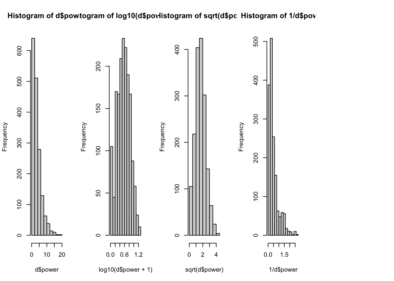
DISCORD DISCUSSION : Below are these three transformations applied to our measure of power words.
What do you see?
Which transformation seems the best to apply to our linear model? (And why?)
A t-test does compares this difference between groups (our slope) to an estimate of sampling error.
\[
t = b / se
\]
Sampling Error.
Previously, we’ve estimated sampling error using bootstrapping.
## Sampling Error (Bootstrapping)bucket <-array()for(i inc(1:1000)){ dboot <- d[sample(1:nrow(d), nrow(d), replace = T), ] modboot <-lm(power ~ pocuF, data = dboot) bucket[i] <-coef(modboot)[2]}mean(bucket) # should be close to original model
[1] 0.4794735
sd(bucket) # the estimate of sampling error
[1] 0.1414262
The Standard Error.
The standard error estimates how much of a difference we might find if we were drawing a random sample from a population where there was no difference in groups (the null population.)
The basic equation for the standard error is :\(se = sd(x) / \sqrt{n}\)
You can calculate this “by hand” if you’d like.
## Pooling the SDd0 <- d[d$pocuF =="Authors of Color",]d1 <- d[d$pocuF =="White Authors",]## calculating the sample size of these two new datasets.n0 <-nrow(d0)n1 <-nrow(d1)df0 <- n0-1# the sample size, minus 1df1 <- n1-1var0 <-var(d0$power)var1 <-var(d1$power)poolvar <- ((df1 * var1) + (df0 * var0))/(df1 + df0)sqrt((poolvar/n0) + (poolvar/n1))
[1] 0.1513899
However, most students and researchers do not like to do things by hand. And so we can easily pull up these statistics using the summary() function. The interpretation of these statistics will take more time!
summary(mod)
Call:
lm(formula = power ~ pocuF, data = d)

Residuals:
    Min      1Q  Median      3Q     Max
-3.5632 -2.0955 -0.7677  1.2943 14.9068

Coefficients:
                   Estimate Std. Error t value Pr(>|t|)
(Intercept)          3.0722     0.1254  24.491   <2e-16 ***
pocuFWhite Authors   0.4910     0.1514   3.243   0.0012 **
---
Signif. codes:  0 '***' 0.001 '**' 0.01 '*' 0.05 '.' 0.1 ' ' 1

Residual standard error: 2.885 on 1686 degrees of freedom
Multiple R-squared:  0.006201,  Adjusted R-squared:  0.005612
F-statistic: 10.52 on 1 and 1686 DF,  p-value: 0.001204
Standard Error is similar to the sampling error we estimated through bootstrapping.1
1 (And side note : to get what R calculates in our model, we will weight each pooled variance by the sample size of each group.)
summary(mod)$coefficients[2,2] # pulling out the standard error of the slope.
[1] 0.1513899
sd(bucket) # pretty close!! wow!!!!
[1] 0.1414262
Conceptual and Computational Differences Between NHST and Bootstrapping
we want to estimate how much our statistics might change due to re-sampling, because our sample isn’t a perfect representation of the population.
we generate lots of “new” samples from our original dataset. these new samples are the same size as our original sample, but we use sampling with replacement to make sure we don’t get the exact same people in the sample every time. the goal is to see how small changes to our sample (that we might find with sampling error) influence our results (the model).
we calculate a statistic that is based on:
the variance in our sample (with the idea that the more individuals vary in the sample, the more sampling error we might have)
our sample size (with the idea that the larger our sample, the less sampling error we will find.)
statistic we care about that defines sampling error
standard deviation of the 1,000 (or however many) slopes we generated from bootstrapping.
standard error (estimates how much the average slope would differ from b = 0….the expected slope assuming the null)
how to evaluate our slope, relative to sampling error
calculate the % of slopes in the same direction as our slope
calculate 95% confidence intervals, and see whether that range includes zero and / or numbers in the opposite direction of the slope you found. (e.g., if you found a negative number, does the range include positive numbers? If so, then likely we’d find a positive relationship due to chance)
t-value : evaluates slope you found, relative to slope you might find due to random chance.
use the t-value to calculate the probability given your distribution, and reject if p < .05
(or be more conservative and reject if p < .01 or p < .001).
Yes, professor, but I learned about t-tests as their own thing?
Note that the t-test does the same thing that our linear model does; evaluates the difference in groups, relative to an estimate of the sampling error we might observe.
t.test(d0$power, d1$power, var.equal = T)
Two Sample t-test
data: d0$power and d1$power
t = -3.2435, df = 1686, p-value = 0.001204
alternative hypothesis: true difference in means is not equal to 0
95 percent confidence interval:
-0.7879644 -0.1941005
sample estimates:
mean of x mean of y
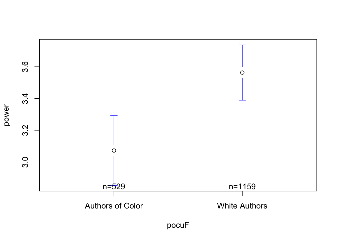
3.072212 3.563244
Comments on the Mid-Semester Evaluation
ideas for changes
other comments :