Class 12 - The End

Check-In : The Learning Has Stopped (Long Live The Learning)

Announcements :

• Final Project Due.

• Next Week : Virtual RRR Time (on Zoom) 11-????

• Outstanding Grades : prof will do ASAP

  • Brain Exam

  • Discussion Posts

  • Discussion Presentations

  • Attendance / Check-Ins.

Part 1 : More MLM (or, in this case, “Linear Mixed Model”)

Example 1 : Another sleepstudy

A classic teaching dataset from lmer. Hooray!

library(lme4)

Loading required package: Matrix

?sleepstudy
s <- sleepstudy

A Question : Is there a relationship between number of days of sleep deprivation and reaction time?

The Graph

How might we graph this in ggplot?

library(ggplot2)
ggplot(sleepstudy, aes(y = Reaction, x = Days, color = Subject)) + 
  geom_point(size=2) + 
  # facet_wrap(~Subject) + 
  geom_smooth(method = "lm")

`geom_smooth()` using formula = 'y ~ x'

  # geom_line(aes(group = Subject), linewidth = 0.75)

Interpreting the Model (Random Intercepts)

What model would we define?

• Reaction is the DV

• I’m adding Days as a Fixed IV (so I’ll get the average effect of # of days of sleep deprivation on reaction time)

• I’m also adding a random intercept : (1 | Subject) that will estimate how much the intercept (the 1 term) of individual raction times (the level 2 variable) varies by Subject (the level 1 grouping variable).

library(lme4)
l2 <- lmer(Reaction ~ Days + (1 | Subject), data = sleepstudy)
summary(l2)

Linear mixed model fit by REML ['lmerMod']
Formula: Reaction ~ Days + (1 | Subject)
   Data: sleepstudy

REML criterion at convergence: 1786.5

Scaled residuals: 
    Min      1Q  Median      3Q     Max 
-3.2257 -0.5529  0.0109  0.5188  4.2506 

Random effects:
 Groups   Name        Variance Std.Dev.
 Subject  (Intercept) 1378.2   37.12   
 Residual              960.5   30.99   
Number of obs: 180, groups:  Subject, 18

Fixed effects:
            Estimate Std. Error t value
(Intercept) 251.4051     9.7467   25.79
Days         10.4673     0.8042   13.02

Correlation of Fixed Effects:
     (Intr)
Days -0.371

How do we interpret the results of this model?

• Fixed Effects : these deal with the “average” effects - ignoring all those important individual differences (which are accounted for in the random effects.)

  • Intercept = 251.41 = the average person’s reaction time at 0 days of sleep deprivation is 251.4 milliseconds.

  • Days = 10.47 = for every day of sleep deprivation, the average person’s reaction time increases by 10.47 MS; the standard error is an estimate of how much variation we’d expect in this average slope due

• Random Effects : these describe those individual differences in people’s starting responses to the DV (random intercepts) and individual differences in the relationship between the IV and the DV (random slopes).

  • Subject (Intercept) = 37.12

  • Residual = 30.99

Interpreting the Model (Random Intercepts and Slopes)

What model would we define?

lmer(Reaction ~ Days + (Days | Subject), data = sleepstudy)

Linear mixed model fit by REML ['lmerMod']
Formula: Reaction ~ Days + (Days | Subject)
   Data: sleepstudy
REML criterion at convergence: 1743.628
Random effects:
 Groups   Name        Std.Dev. Corr
 Subject  (Intercept) 24.741       
          Days         5.922   0.07
 Residual             25.592       
Number of obs: 180, groups:  Subject, 18
Fixed Effects:
(Intercept)         Days  
     251.41        10.47  

How do we interpret the results of this model?

Example 2 : Nature and Pain

• ICE BREAKER : what’s your favorite place in the bay area to see nature?

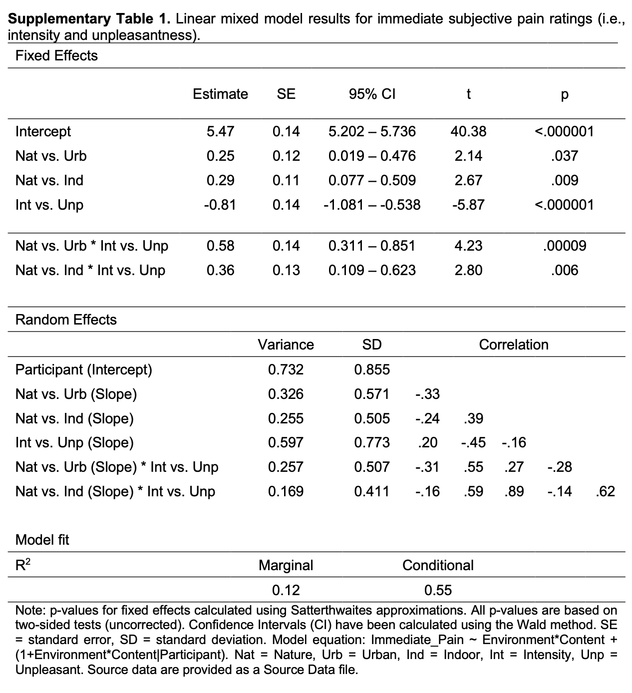
• THE STUDY : participants were shocked while looking at images (virtual nature, urban, or indoor) while getting their brains scanned. participants rated the subjective unpleasantness of each trial.

• THE TABLE :

  • What is going on with this models?

  • What seems important?

  • What seems irrelevant?

  • What questions do you have?

Abstract [full article]	Linear Model Table [link to SI materials]

Part 2 : Final Project Show and Tell

• Find a Buddy.

  • Walk them through your study!

    • What is your question (and why should we care)?

    • How did you measure / manipulate these variables?

  • Walk them through your graph / results!

• Some volunteers to share with the class? Low-stakes practice for more stressful situations where you will be more prepared :)

Common Statistical Mistakes. Any you are doing? Questions?? Feeling the pressure???

1. Absence of an adequate control condition/group

2. Interpreting comparisons between two effects without directly comparing them

3. Spurious correlations

4. Inflating the units of analysis

5. Correlation and causation

6. Use of small samples

7. Circular analysis

8. Flexibility of analysis

9. Failing to correct for multiple comparisons

10. Over-interpreting non-significant results

Part 3 : Would You Like to Learn More?

Watch Out for Overfitting in Your Models

When your model is too complex, each variable in the model (parameter) increases the model complexity.

• ACTIVITY : Where would you draw the line of best fit here?

library(ggplot2)
# Fakin' some data.
set.seed(42)
n <- 100
x <- seq(-5, 5, length.out = n)
y <- sin(x) + rnorm(n, sd = 2)
d <- data.frame(x, y)

# Graphin the fake data.
ggplot(d, aes(x, y)) +
  geom_point(size = 2) +
  # stat_smooth(method = "lm", formula = y ~ poly(x, 25), se = FALSE, color = "red", size = 2) +
  # labs(title = "Overfit Model (25-Degree Polynomial IV") +
  theme_minimal()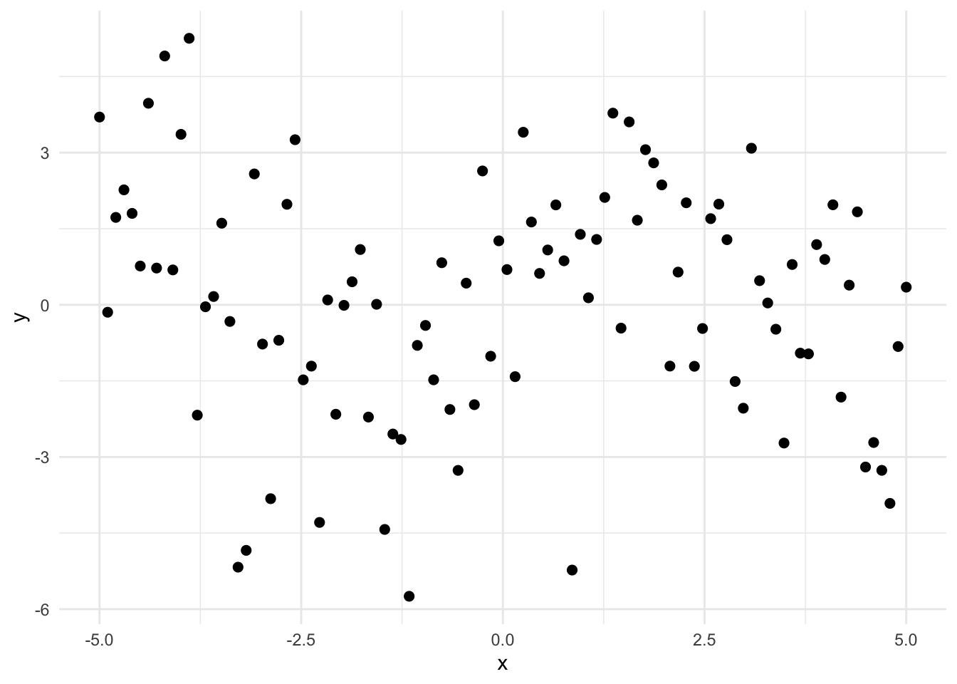

• KEY IDEA : complex models that perfectly fit the data are problematic

  • You essentially describing your sample, and not the underlying population (which is usually the goal of multiple regression.)

• We don’t expect over-fit models to generalize to other samples. [Image source]

  

Cross Validation : Conceptual Understanding

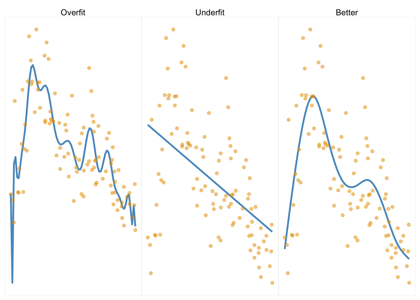
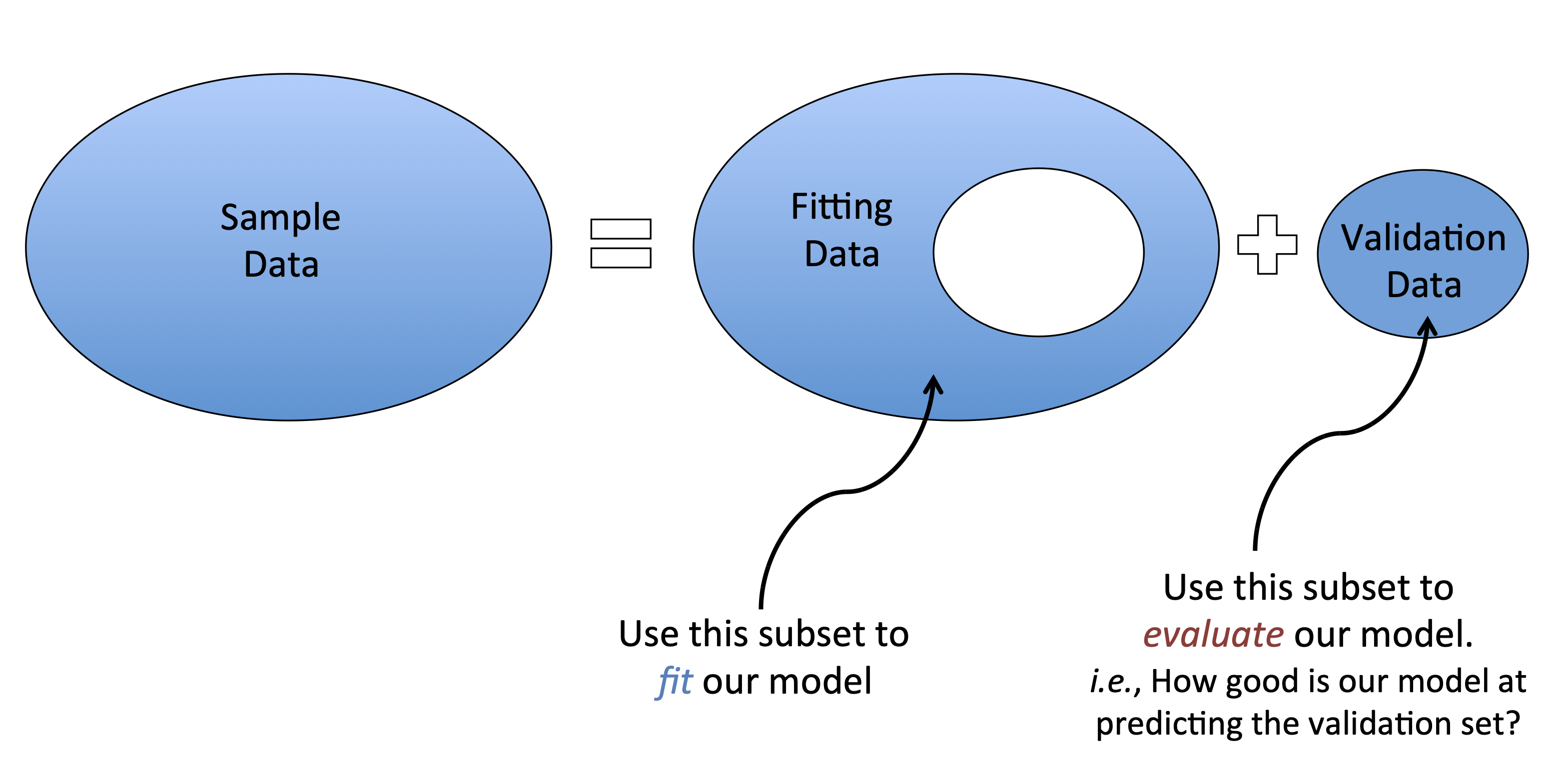
Cross Validation. To ensure your model generalizes to other samples, you can a) replicate, or b) cross-validate your data. Cross validation involves dividing your sample into sub-samples; define a model on one sample, then test the model in the other(s).

Example : Cross-Validating an Interaction Effect

The Graph : The Relationship Between Social Support and Happiness Depends on GDP

h <- read.csv("~/Dropbox/!GRADSTATS/Datasets/World Happiness Report - 2024/World-happiness-report-2024.csv", stringsAsFactors = T)
library(ggplot2)
library(jtools)

## Some data cleaning.
h$GDPcat <- ifelse(scale(h$Log.GDP.per.capita) > sd(h$Log.GDP.per.capita, na.rm = T), "High GDP", "Low GDP")
h$GDPcat <- as.factor(h$GDPcat)
# plot(h$GDPcat) # making sure this re-leveling worked.
ggplot(data = subset(h, !is.na(h$GDPcat)), aes(y = scale(Ladder.score), x = scale(Social.support), color = GDPcat)) + 
  geom_point(alpha = .5, position = "jitter") +
  geom_smooth(method = "lm") + labs(title = "Graph of an Interaction Effect from Lecture 10") + xlab("Social Support") + ylab("Happiness (Ladder Score)") +
  theme_apa()

`geom_smooth()` using formula = 'y ~ x'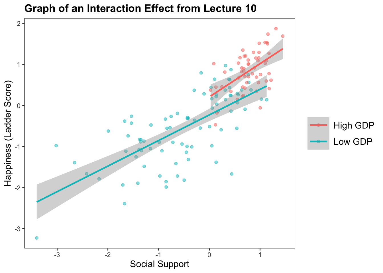

Table : Linear Models for the Interaction Effect from Lecture 10

mod1 <- lm(scale(Ladder.score) ~ scale(Log.GDP.per.capita), data = h)
mod2 <- lm(scale(Ladder.score) ~ scale(Social.support), data = h)
mod3 <- lm(scale(Ladder.score) ~ scale(Log.GDP.per.capita) + scale(Social.support), data = h)
mod4 <- lm(scale(Ladder.score) ~ scale(Social.support) * scale(Log.GDP.per.capita), data = h)
export_summs(mod1, mod2, mod3, mod4)

	Model 1	Model 2	Model 3	Model 4
(Intercept)	0.00	0.00	0.00	-0.09
	(0.05)	(0.05)	(0.04)	(0.06)
scale(Log.GDP.per.capita)	0.78 ***		0.38 ***	0.34 ***
	(0.05)		(0.07)	(0.07)
scale(Social.support)		0.82 ***	0.55 ***	0.64 ***
		(0.05)	(0.07)	(0.07)
scale(Social.support):scale(Log.GDP.per.capita)				0.13 *
				(0.06)
N	140	140	140	140
R2	0.59	0.66	0.73	0.74
*** p < 0.001; ** p < 0.01; * p < 0.05.

Here’s the most simple example of cross-validation (“train-test split”; “holdout cross validation”)

sample(0:1, nrow(h), replace = T, prob = c(.7, .3)) # using the sample function

  [1] 1 0 0 0 1 0 0 0 0 0 0 0 0 1 0 0 0 1 0 0 0 1 0 1 0 0 0 0 0 0 0 0 1 1 0 1 0
 [38] 0 0 0 0 0 0 0 0 0 0 1 0 0 0 0 0 1 0 0 0 0 1 0 0 1 0 0 1 0 1 1 0 1 0 0 1 0
 [75] 0 0 0 0 0 0 0 1 0 0 0 0 0 0 1 1 0 0 0 0 1 0 0 0 0 0 0 0 1 1 0 0 0 0 0 1 0
[112] 0 0 1 0 0 1 1 0 0 0 0 0 1 0 1 1 1 1 0 0 0 0 0 0 0 1 0 0 0 1 0 0

set.seed(424242)
random.selection <- sample(0:1, nrow(h), replace = T, prob = c(.7, .3))
htrain <- h[random.selection == 0,]
htest <- h[random.selection == 1,]

## Model in training Data
train.mod <- lm(Ladder.score ~ Social.support * Log.GDP.per.capita, data = htrain)
summary(train.mod)

Call:
lm(formula = Ladder.score ~ Social.support * Log.GDP.per.capita, 
    data = htrain)

Residuals:
    Min      1Q  Median      3Q     Max 
-1.6407 -0.3823  0.0727  0.3667  1.2845 

Coefficients:
                                  Estimate Std. Error t value Pr(>|t|)    
(Intercept)                         3.3152     0.8238   4.024 0.000133 ***
Social.support                      0.7625     0.7030   1.085 0.281444    
Log.GDP.per.capita                 -0.3721     0.8248  -0.451 0.653165    
Social.support:Log.GDP.per.capita   1.1410     0.6266   1.821 0.072497 .  
---
Signif. codes:  0 '***' 0.001 '**' 0.01 '*' 0.05 '.' 0.1 ' ' 1

Residual standard error: 0.6336 on 77 degrees of freedom
  (2 observations deleted due to missingness)
Multiple R-squared:  0.7538,    Adjusted R-squared:  0.7442 
F-statistic: 78.57 on 3 and 77 DF,  p-value: < 2.2e-16

predict(train.mod) # the predicted values of the DV, based on our model.

       1        2        4        6        7        8        9       10 
7.135230 7.073353 6.977285 6.893786 7.124321 6.861858 6.871832 6.829994 
      12       13       17       18       19       20       21       22 
6.226749 6.540176 6.959481 6.877903 6.696600 6.404965 6.856755 6.098574 
      24       29       31       34       35       37       38       39 
6.646297 5.768824 6.485067 6.880177 6.558980 6.244588 6.282021 6.446558 
      41       42       44       46       51       53       54       55 
6.385499 5.418369 5.821278 6.757584 6.442304 5.341571 5.710209 6.412559 
      58       60       61       63       65       67       68       70 
6.070923 5.819241 4.986850 6.600110 5.978203 5.782169 5.550716 6.199191 
      74       75       79       84       85       86       87       89 
5.430531 5.825515 4.322492 5.889255 5.529930 6.086642 5.000752 4.090630 
      91       93       94       97       98       99      101      102 
5.181336 4.801076 4.676863 4.070036 5.859680 4.337256 4.882258 5.025275 
     104      105      108      110      111      112      114      116 
4.538053 5.841144 4.106776 4.147098 4.318803 4.143023 4.670770 3.206190 
     117      119      120      121      122      123      127      128 
4.919463 4.891486 4.402009 4.073373 4.148257 4.298796 5.121814 5.538658 
     129      130      132      133      134      140      141      142 
3.406342 4.545065 3.567231 5.023060 4.427402 3.925790 4.425851 4.149352 
     143 
3.081519 

## Applying the model to our testing dataset.
predict(train.mod, newdata = htest) # produces predicted values from our training model, using the testing data.

       3        5       11       14       15       16       23       25 
7.318721 6.910581 6.959649 6.505973 6.806142 6.787351 6.734791 5.849235 
      26       27       28       30       32       33       36       40 
6.418403 6.462812 6.528031 6.853932 6.021541 5.226853 6.743818 6.746631 
      43       45       47       48       49       50       52       56 
5.450941 6.852365 5.854924 6.248302 6.519124 6.066788 5.977630 6.841798 
      57       59       64       66       69       71       72       73 
6.114564 5.720941 6.113327 5.501434 5.922356 5.791608 6.265510 5.398525 
      76       77       78       80       81       82       83       90 
6.098167 6.296563 5.761549 5.550235 6.559611 5.559175 6.011906 4.344333 
      92       95       96      100      103      106      107      109 
5.029329 5.246298 4.066328 5.507476       NA 5.519041 3.874870 4.060831 
     113      115      118      124      125      126      131      135 
4.258512 4.980537 4.807166 3.986804 5.010633 4.248014 4.208966 4.878107 
     136      137      138      139 
3.686886 5.114035 4.410461 4.028756 

predval.test <- predict(train.mod, newdata = htest)  # saves these predicted values from the testing dataset.

## Calculating R^2
test.mod.resid <- htest$Ladder.score - predval.test
SSE <- sum(test.mod.resid^2, na.rm = T)
SSE

[1] 19.87085

test.resid <- htest$Ladder.score - mean(htest$Ladder.score, na.rm = T)
SST <- sum(test.resid^2, na.rm = T)
(SST - SSE)/SST

[1] 0.7104798

Interpreting Cross Validation

You’ll often see a few different methods of evaluating model fit.

• \(R^2\). Our good friend. The proportion of variance explained by the model (vs. the mean)
• Rooted Mean Squared Error (RMSE). The average amount of residual error (actual - predicted values).
• Mean Absoulte Error. The average of the absolute value of the residuals; less sensitive to outliers than RMSE or \(R^2\).

And there are different methods of defining the test and training datasets. And different packages and tutorials to do this.

Here’s one, called “Leave one out cross validation - LOOCV”; gif below via Wikipedia.

# install.packages("caret")
library(caret)

Loading required package: lattice

train.control <- trainControl(method = "LOOCV")
loocvmod <- train(Ladder.score ~ Social.support * Log.GDP.per.capita, data = h, method = "lm",
                  trControl = train.control, na.action = "na.omit")
print(loocvmod)

Linear Regression 

143 samples
  2 predictor

No pre-processing
Resampling: Leave-One-Out Cross-Validation 
Summary of sample sizes: 139, 139, 139, 139, 139, 139, ... 
Resampling results:

  RMSE       Rsquared   MAE      
  0.6342914  0.7098648  0.4796968

Tuning parameter 'intercept' was held constant at a value of TRUE

Watch Out for Multicollinearity.

If your independent variables are highly related, then your multivariate regression slope estimates are not uniquely determined. weird things happen to your coefficients, and this makes it hard to interpret your effects.

• IN R : check the “variance inflation factor” (VIF); a measure of how much one IV is related to all the other IVs in the model. “Tradition” is that if VIF is > 5 (or I’ve also seen VIF > 10) there’s a problem in the regression.

• \(\huge VIF_j=\frac{1}{1-R_{j}^{2}}\)

library(car)

Loading required package: carData

vif(mod4) # doesn't seem like multicollinearity is a problem.

there are higher-order terms (interactions) in this model
consider setting type = 'predictor'; see ?vif

                          scale(Social.support) 
                                       2.847840 
                      scale(Log.GDP.per.capita) 
                                       2.222549 
scale(Social.support):scale(Log.GDP.per.capita) 
                                       1.433238 

## creating a highly correlated second IV for the sake of this example.
jitter(h$Healthy.life.expectancy, 300)

  [1]  0.63649887  0.68930612  0.71828952  0.66823278  0.78147940  0.64639281
  [7]  0.66783200  0.65547462  0.71468602  0.72225337  0.71773673  0.64999642
 [13]  0.62952106  0.64185465  0.72092831  0.69836634  0.64067483  0.60323449
 [19]  0.61564585  0.70589567  0.74527554  0.54082440  0.57966955  0.74032124
 [25]  0.52293196  0.54462176  0.75101008  0.55563685  0.60367356  0.74810486
 [31]  0.69789473  0.54448689  0.56294229  0.69718620  0.62746987  0.69055692
 [37]  0.62267421  0.70380172  0.62007029  0.68723153  0.74690172  0.49826800
 [43]  0.58734907  0.50056514  0.69238462  0.52731539  0.57692015  0.64389105
 [49]  0.57280871  0.69425428  0.82612563  0.77274534  0.38400182  0.57725457
 [55]  0.70352020  0.61930331  0.55762718  0.57337490  0.53553203  0.65959492
 [61]  0.45026458          NA  0.66845212  0.69307250  0.59281784  0.52861070
 [67]  0.54621673  0.69875356  0.45710762  0.43500797  0.56482900  0.54559839
 [73]  0.50964668  0.60188374  0.54674710  0.60113762  0.41675213  0.67774238
 [79]  0.45482879  0.51207586  0.53754193  0.65166685  0.26579890  0.58060330
 [85]  0.53234986  0.85807969  0.66611649          NA  0.25647428  0.12829974
 [91]  0.51774245  0.49561179  0.47517286  0.47895859  0.35411168  0.25447142
 [97]  0.21655523  0.58171885  0.35686944  0.51373138  0.48182973  0.20760587
[103]          NA  0.31835400  0.46658725  0.34832926  0.52310604  0.28958395
[109]  0.33832352  0.33133514  0.42088085  0.27791840  0.16285129  0.31895572
[115]  0.62433954  0.30866350  0.37751970  0.43665557  0.41469131  0.38656597
[121]  0.32196352  0.25386893  0.35348747  0.26579842  0.62022055  0.43845057
[127]  0.49687114  0.62927456  0.48772773  0.38520825  0.37719937  0.40156511
[133]  0.33585422  0.29027768  0.12197319  0.39450247  0.18769012  0.21595348
[139]  0.24276263  0.24909294 -0.03799866  0.57172747  0.27471988

h$health2 <- jitter(h$Healthy.life.expectancy, 300)

plot(h$health2, h$Healthy.life.expectancy) # yup.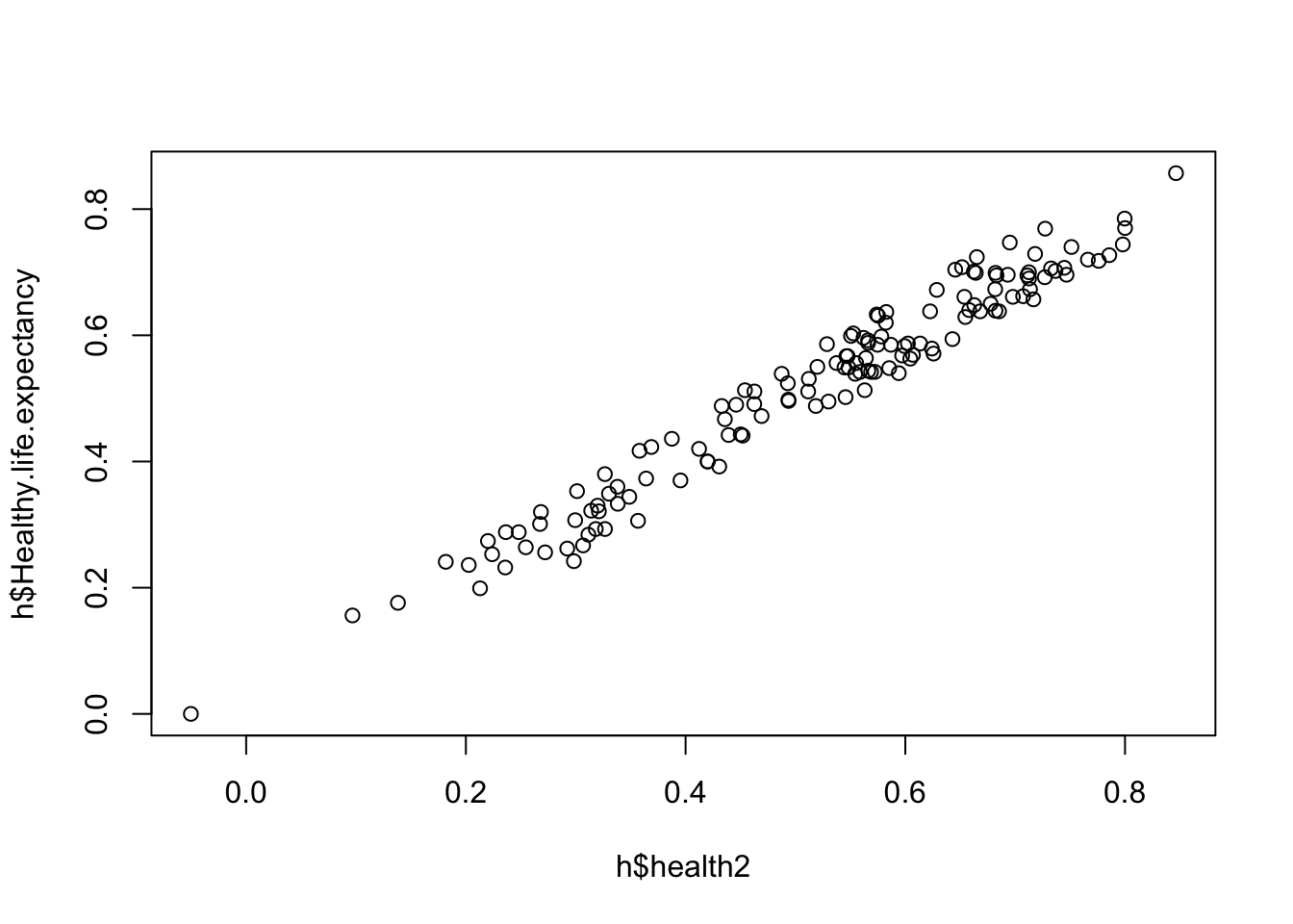

multimod <- lm(Ladder.score ~ Healthy.life.expectancy + health2, data = h) # both in the model.
summary(multimod) # results! Things look good....

Call:
lm(formula = Ladder.score ~ Healthy.life.expectancy + health2, 
    data = h)

Residuals:
    Min      1Q  Median      3Q     Max 
-3.0155 -0.4313  0.1701  0.5191  1.5809 

Coefficients:
                        Estimate Std. Error t value Pr(>|t|)    
(Intercept)               2.6514     0.2202  12.041  < 2e-16 ***
Healthy.life.expectancy   7.5885     1.9725   3.847 0.000182 ***
health2                  -2.0676     1.8604  -1.111 0.268360    
---
Signif. codes:  0 '***' 0.001 '**' 0.01 '*' 0.05 '.' 0.1 ' ' 1

Residual standard error: 0.7703 on 137 degrees of freedom
  (3 observations deleted due to missingness)
Multiple R-squared:  0.5809,    Adjusted R-squared:  0.5747 
F-statistic: 94.93 on 2 and 137 DF,  p-value: < 2.2e-16

vif(multimod) # ...but wait!

Healthy.life.expectancy                 health2 
               24.78939                24.78939 

Things to Read!

• An overview of ML methods (including the partitioning approach) for evaluating models
• Another overview of cross-validation methods.
• Some more notes on multicollinearity and VIFs.

A Discussion on Effect Size and the Course and Psychology

There’s a LOT of Error in Our Predictions of People.

Richard, F. D., Bond Jr, C. F., & Stokes-Zoota, J. J. (2003). One hundred years of social psychology quantitatively described. Review of general psychology, 7(4), 331-363.

But Life, In General, is Complex

• ARTICLE : Meyer, G. J., Finn, S. E., Eyde, L. D., Kay, G. G., Moreland, K. L., Dies, R. R., Eisman, E.J., Kubiszyn, & Reed, G. M. (2001). Psychological testing and psychological assessment: A review of evidence and issues. American psychologist, 56(2), 128.

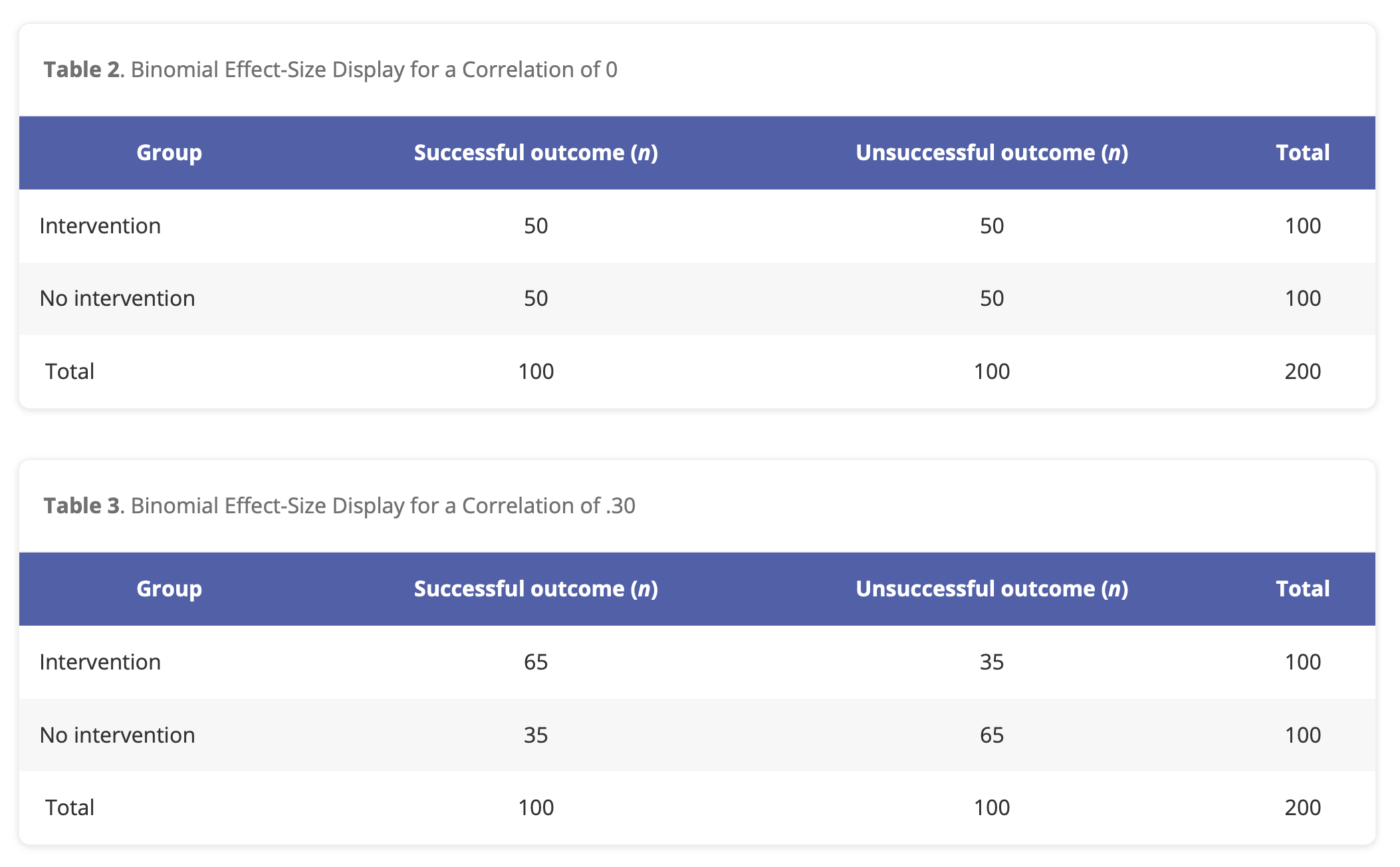
• ACTIVITY :

  • Find a “Hard Science” effect from Table 1. Does the size of this correlation surprise you? Why / why not?

  • Find a “Psych Science” effect from Table 2. Does the size of this correlation surprise you? Why / why not?

Small Effects Matter

• Funder DC, Ozer DJ. Evaluating Effect Size in Psychological Research: Sense and Nonsense. Advances in Methods and Practices in Psychological Science. 2019;2(2):156-168. doi:10.1177/2515245919847202

Doing Good Science is Hard But Important to Be “Valid”

• Allen C, Mehler DMA (2019) Correction: Open science challenges, benefits and tips in early career and beyond. PLOS Biology 17(12): e3000587. https://doi.org/10.1371/journal.pbio.3000587

Percentages of null findings among RRs and traditional (non-RR) literature [46,47], with their respective 95% confidence intervals.

Other Methods Exist for Describing the World

1. Qualitative studies.
2. Philosophy.
3. Critical Theory.
4. History.
5. Art.
6. Religion / faith.

What are the Benefits of Using the Scientific Approach? What are the Limitations (or Dangers)?

Is a “Valid” Psychological Science Possible?

^{_{Farewell! Feel free to stay in touch :) it has been a pleasure and privilege to work with y’all this semester <3}}